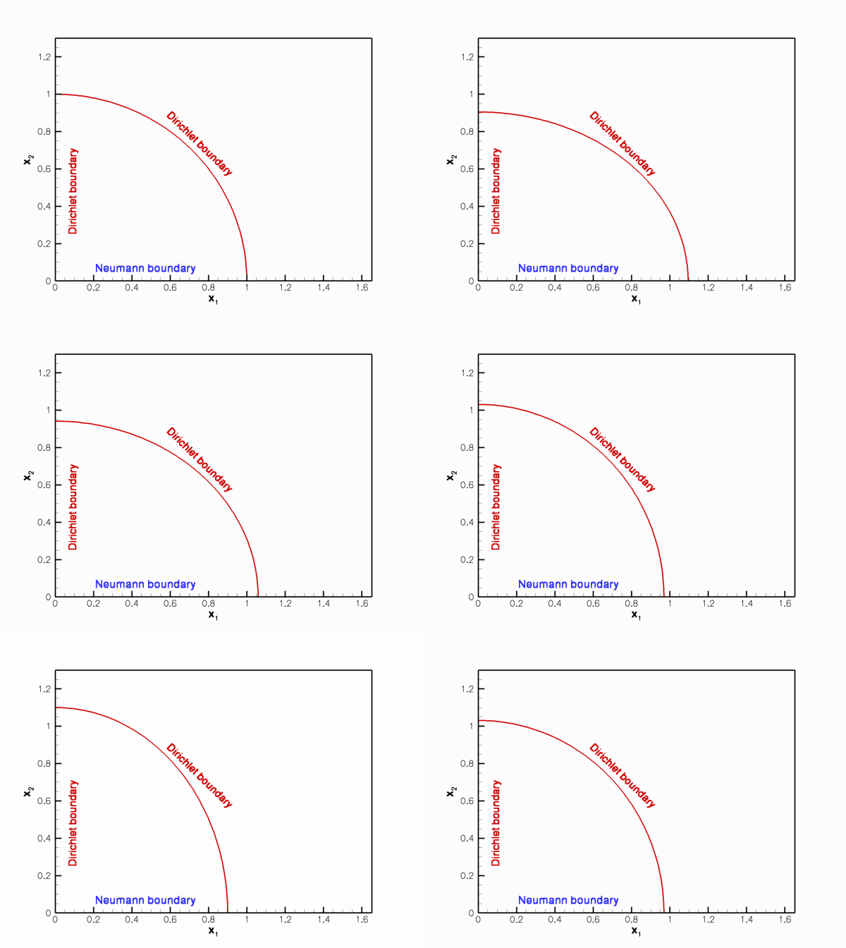
In this example we consider the solution of the unsteady heat equation in a domain with moving boundaries. We demonstrate that the presence of moving boundaries only requires trivial changes to driver codes for corresponding fixed-mesh computations.

The two-dimensional unsteady heat equation with flux boundary conditions in a moving domain. Solve

$\sum_{i=1}^2\frac{\partial^2 u}{\partial x_i^2} = \frac{\partial u}{\partial t} + f\left(x_1,x_2,t\right), \ \ \ \ \ \ \ \ \ \ (1)$

in the domain

, bounded by the coordinate axes and the time-dependent ellipse

$\mathbf{r}_{ellipse}(\xi,t) = \left( \begin{array}{c} \big( a+\hat{a}\sin(2\pi t/\hat{T}) \big) \cos(\xi) \\ \big( b+\hat{b}\sin(2\pi t/\hat{T}) \big) \sin(\xi) \end{array} \right), \ \ \ \ \ \ \ \ \ \ (2)$

subject to Neumann boundary conditions,

$\left. \frac{\partial u}{\partial n}\right|_{\partial D_{Neumann}}= - \left. \frac{\partial u}{\partial x_2}\right|_{\partial D_{Neumann}}= g_0, \ \ \ \ \ \ \ \ \ \ (3)$

along the horizontal domain boundary $\partial D_{Neumann} = \{ (x_1,x_2) | x_1 \in [0,1], x_2=0 \}$ , and to Dirichlet boundary conditions,

$\left. u\right|_{\partial D_{Dirichlet}}=h_0, \ \ \ \ \ \ \ \ \ \ (4)$

elsewhere.

Sketch of the time-dependent domain and the boundary conditions.

The initial conditions are given by

$u(x_1,x_2,t=0)=k_0(x_1,x_2), \ \ \ \ \ \ \ \ \ \ (5)$

where the functions $f, g_0, \ h_0$ and

are given.

We choose the functions $f, g_0, \ h_0$ and so that

$u_0(x_1,x_2,t) = \tanh\bigg[ 1-\alpha\bigg( \tan\Phi \big(x_1-\beta\tanh[ \gamma\cos\left(2\pi t\right)]\big)- x_2\bigg)\bigg] \ \ \ \ \ \ \ \ \ \ (6)$

is the exact solution.

The solution represents the "usual" tanh profile, whose steepness is controlled by the parameter $\alpha$ so that for $\alpha \gg 1$ the solution approaches a step. The step is oriented at an angle $\Phi$ against the axis and its position varies periodically. The parameter $\beta$ controls the amplitude of the step's lateral displacement, while $\gamma$ determines the rate at which its position changes. For $\gamma \gg 1$ , the step remains stationary for most of the period and then translates rapidly parallel to the axis, making this a very challenging problem.

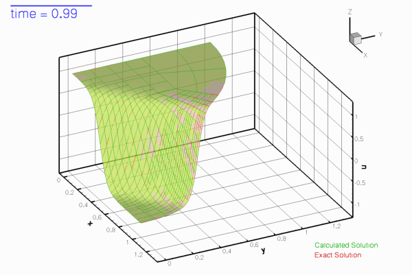
The figure below shows a snapshot of the animated solution, obtained from the spatially adaptive simulation discussed below, for the parameter values $\alpha=10, \ \Phi=45^o, \ \beta=-0.3, \ \gamma=5.$

Snapshot of the solution.

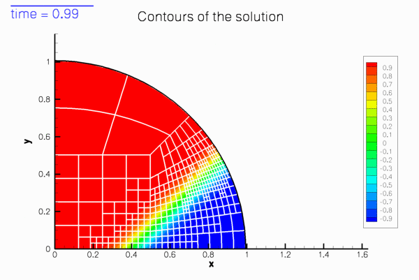
The mesh adaptation in response to the translation of the step can be seen more clearly in this contour plot, taken from another animation of the solution.

Contour plot of the solution.

Background: ALE methods and the evaluation of time-derivatives in moving domains

oomph-lib's UnsteadyHeatEquations, the equation class that forms the basis for the isoparametric QUnsteadyHeatElements, is based on the Arbitrary Lagrangian Eulerian (ALE) formulation of the weak form of the governing PDE, (1). Within each element, the solution is represented by interpolation between the element's $N_{node}^{(E)}$ nodal values $U_j^{(E)}(t) \ (i=1,..., N_{node}^{(E)})$ , i.e.

$u = \sum_{j=1}^{N_{node}^{(E)}} U_j^{(E)}(t) \ \psi_{j}(s_1,s_2), \ \ \ \ \ \ \ \ \ \ (7)$

where and are the element's two local coordinates. The mapping between the local and global (Eulerian) coordinates is based on the interpolation between the nodal coordinates,

$x_i(s_1,s_2) = \sum_{j=1}^{N_{node}^{(E)}} X_{ij}^{(E)}(t) \ \psi_{j}(s_1,s_2), \ \ \ \ (i=1,2) \ \ \ \ \ \ (8)$

where $X_{ij}^{(E)}(t)$ is the i-th global (Eulerian) coordinate of node j in the element. In moving-domain problems, where the nodal positions vary as function of time, the time-derivative of the nodal value, , represents the rate-of-change of at the moving node, rather than the time-derivative of at a fixed Eulerian position,
$\partial u/\partial t,$ the quantity required in the PDE, (1).

The rate of change of at a moving node, , may also be expressed by the material derivative,

$\left. \frac{D u}{Dt}\right|_{\mbox{\small node} \ j} = \frac{\partial u}{\partial t} + \sum_{i=1}^2 v_{ij} \ \frac{\partial u}{\partial x_i}$

where

$v_{ij} = \frac{dX_{ij}^{(E)}}{dt}$

is the i-th velocity component of node j, often referred to as the "mesh velocity". The rate of change of , experienced at the (fixed) spatial position that coincides with the current position of node j is therefore given by

$\frac{\partial u}{\partial t} = \frac{d U_j^{(E)}}{dt} - \sum_{i=1}^2 \left( \frac{dX_{ij}^{(E)}}{dt} \ \sum_{k=1}^{N_{node}^{(E)}} U_k^{(E)} \ \frac{\partial \psi_{k}}{\partial x_i} \right) .$

This is the form in which the time-derivative in (1) is implemented in oomph-lib's unsteady heat elements. The mesh velocity is determined automatically, using the Node's positional TimeStepper and the history values of the nodal positions. [By default, the positional TimeStepper is the same as the TimeStepper used for the evaluation of the time-derivatives of the nodal values; a different one may be assigned with the access function Node::position_time_stepper_pt().] This is why it is important to initialise the "previous nodal positions" in computations on fixed meshes, as demonstrated in the exercise in our earlier example: The previous nodal positions are initialised to zero when a Node is first created. Therefore, if the previous positions are not overwritten with the actual nodal positions, the positional TimeStepper would compute non-zero mesh velocities, even though the Nodes are stationary.

oomph-lib's unsteady Newton solvers automatically advance the time-history of the nodal positions when computing a new timestep. Performing computations on moving meshes is therefore extremely straightforward: The only task to be performed by the "user" is to update the nodal positions before a new timestep is taken. This is best done in the function Problem::actions_before_implicit_timestep().

The update of the nodal positions may be performed "manually", by assigning new nodal positions directly, using the function Node::x(...). However, in most cases, the deformation of the domain will be driven by the motion of its boundaries. We discussed in an earlier example, that in oomph-lib curvilinear, moving boundaries are typically represented by (time-dependent) GeomObjects which define the MacroElement boundaries of the Domain object associated with the Mesh. In this case, the update of the nodal positions may be performed by updating the parameters that control the shape of the GeomObject and calling the Mesh's node-update function Mesh::node_update(), as illustrated in the earlier example.

It is also possible (and, in fact, much easier) to include the time-dependence of the domain boundaries into the definition of the GeomObject, by making its shape, described by GeomObject::position(...), a function of time. In that case, the update of the nodal positions in response to the boundary motion merely requires a call to Mesh::node_update() in Problem::actions_before_implicit_timestep(). This is the approach we take in the present problem.

Global parameters and functions

As usual, we store the problem parameters in a namespace, TanhSolnForUnsteadyHeat, in which we also specify the source function, the prescribed flux along the Neumann boundary and the exact solution. The namespace is identical to that used in the fixed domain example.

Representing the moving curvilinear domain boundary by a time-dependent GeomObject

As discussed above, we will incorporate the time-dependence of the moving curvilinear boundary into the specification of the GeomObject that defines that boundary. For this purpose we represent the elliptical boundary by the GeomObject MyEllipse. Its constructor stores the geometric parameters (the mean values of the ellipse's half axes, and , the amplitude of their temporal variations $\hat{a}$ and $\hat{b}$ , and the period of the oscillation, $\hat{T}$ , in its private member data. We also store a pointer to a Time object to give the GeomObject access to the "current" and "previous" values of the "continuous time". The destructor can remain empty.

//============start_of_MyEllipse===========================================
/// Oscillating ellipse
/// \f[ x = (a + \widehat{a} \sin(2\Pi t/T)) \cos(\xi)  \f]
/// \f[ y = (b + \widehat{b} \sin(2\Pi t/T)) \sin(\xi)  \f]
//=========================================================================
class MyEllipse : public GeomObject
{
 
public:
 
 /// Constructor:  Pass half axes, amplitudes of their variation, period
 /// of oscillation and pointer to time object.
 MyEllipse(const double& a, const double& b, 
           const double& a_hat, const double& b_hat, 
           const double& period, Time* time_pt) : 
  GeomObject(1,2), A(a), B(b), A_hat(a_hat), B_hat(b_hat), 
  T(period), Time_pt(time_pt) {}
 
 /// Destructor: Empty
 virtual ~MyEllipse() {}

The "steady" version of the position(...) function must return the position vector to the point on the GeomObject, identified by its intrinsic coordinate xi, and evaluated at the current value of the continuous time, which we extract from Time::time():

 /// Current position vector to material point at 
 /// Lagrangian coordinate xi 
 void position(const Vector<double>& xi, Vector<double>& r) const
  {
   // Get current time:
   double time=Time_pt->time();
 
   // Position vector
   r[0] = (A+A_hat*sin(2.0*MathematicalConstants::Pi*time/T))*cos(xi[0]);
   r[1] = (B+B_hat*sin(2.0*MathematicalConstants::Pi*time/T))*sin(xi[0]);
 
  } // end of position(...)

The "time-dependent" version of the position(...) function must return the position vector to the GeomObject, evaluated at the t - th previous timestep. The value of the continuous time at that timestep is available from from Time::time(t):

 /// Parametrised position on object: r(xi). Evaluated at
 /// previous time level. t=0: current time; t>0: previous
 /// time level.
 void position(const unsigned& t, const Vector<double>& xi,
               Vector<double>& r) const
  {
   // Get current time:
   double time=Time_pt->time(t);
   
   // Position vector
   r[0] = (A+A_hat*sin(2.0*MathematicalConstants::Pi*time/T))*cos(xi[0]);
   r[1] = (B+B_hat*sin(2.0*MathematicalConstants::Pi*time/T))*sin(xi[0]);
 
  } // end of position(...)

We omit the code that defines the private member data.

The main function

Since the deformation of the domain and the update of the nodal positions will be handled automatically by adding a call to Mesh::node_update() to Problem::actions_before_implicit_timestep(), the driver code for this problem is exactly the same as that in the previous example in a fixed domain.

The Problem class

The Problem class and most of its member functions are exactly the same as in the previous example.

The Problem constructor

The Problem constructor is identical to the fixed-mesh version in the previous example, apart from the fact that we use the MyEllipse GeomObject to define the curvilinear Mesh boundary. Here is the relevant code fragment:

 // Setup mesh
 //-----------
 
 // Build geometric object that forms the curvilinear domain boundary:
 // an oscillating ellipse
 
 // Half axes
 double a=1.0;
 double b=1.0;
 
 // Variations of half axes
 double a_hat= 0.1;
 double b_hat=-0.1;
 
 // Period of the oscillation
 double period=1.0;
 
 // Create GeomObject
 Boundary_pt=new MyEllipse(a,b,a_hat,b_hat,period,Problem::time_pt()); 
 
 // Start and end coordinates of curvilinear domain boundary on ellipse
 double xi_lo=0.0;
 double xi_hi=MathematicalConstants::Pi/2.0;
 
 // Now create the bulk mesh. Separating line between the two 
 // elements next to the curvilinear boundary is located half-way
 // along the boundary.
 double fract_mid=0.5;
 Bulk_mesh_pt = new RefineableQuarterCircleSectorMesh<ELEMENT>(
  Boundary_pt,xi_lo,fract_mid,xi_hi,time_stepper_pt());

Actions before timestep

As discussed above, the addition of a single line to Problem::actions_before_implicit_timestep() suffices to update the nodal positions in response to the changes in the domain boundary.

//=========start of actions_before_implicit_timestep===============================
/// Actions before timestep: Update the domain shape, then set the 
/// boundary conditions for the current time.
//========================================================================
template<class ELEMENT>
void RefineableUnsteadyHeatProblem<ELEMENT>::actions_before_implicit_timestep()
{
 // Update the domain shape
 Bulk_mesh_pt->node_update();

The rest of this function is identical to the that in the fixed-domain version and updates the nodal values on the Dirichlet boundaries according to the values given by the exact solution.

Setting the initial condition

The only other change to the code occurs in the assignment of the initial conditions. The Nodes' positional history values are given by the positions at which the Nodes would have been at previous timesteps. Similarly, the history values themselves must be computed by evaluating the exact solution at the position at which the Nodes would have been at those timesteps.

This is achieved with a few minor changes to the previous version of this function. We loop over the previous timesteps, reconstruct the value of the continuous time at that timestep, and temporarily over-write the value of the continuous time stored in Time::time(). This ensures that the call to MyEllipse::position(...) during the node update operation returns the position vector to the domain boundary at that timestep. Following the update of the nodal positions (which moves them into the position they would have occupied at the previous timestep) we copy their positions and the value of the exact solution into the appropriate history values. Here is the relevant code fragment from the set_initial_condition() function:

   // Loop over current & previous timesteps (in outer loop because
   // the mesh also moves!)
   for (int itime=nprev_steps;itime>=0;itime--)
    {
     double time=prev_time[itime];
     
     // Set global time (because this is how the geometric object refers 
     // to continous time 
     time_pt()->time()=time;
     
     cout << "setting IC at time =" << time << std::endl;
     
     // Update the mesh for this value of the continuous time
     // (The wall object reads the continous time from the same
     // global time object)
     Bulk_mesh_pt->node_update(); 
     
     // Loop over the nodes to set initial guess everywhere
     for (unsigned jnod=0;jnod<num_nod;jnod++)
      {
       // Get nodal coordinates
       x[0]=Bulk_mesh_pt->node_pt(jnod)->x(0);
       x[1]=Bulk_mesh_pt->node_pt(jnod)->x(1);
       
       // Get intial solution
       TanhSolnForUnsteadyHeat::get_exact_u(time,x,soln);
       
       // Assign solution
       Bulk_mesh_pt->node_pt(jnod)->set_value(itime,0,soln[0]);
       
       // Loop over coordinate directions
       for (unsigned i=0;i<2;i++)
        {
         Bulk_mesh_pt->node_pt(jnod)->x(itime,i)=x[i];
        }
      } 
    } // end of loop over previous timesteps

Comments and Exercises

While the spatial adaptivity resolves the rapid spatial variations in the solution, the time-integration with a fixed timestep introduces errors during the phases when the solution undergoes rapid temporal variations. The animations of the exact and computed solutions show clearly that the computed solution lags behind the exact one during these phases. In the next example we will therefore demonstrate how to combine temporal and spatial adaptivity.

Source files for this tutorial

The source files for this tutorial are located in the directory: demo_drivers/unsteady_heat/two_d_unsteady_heat_ALE/
The driver code is: demo_drivers/unsteady_heat/two_d_unsteady_heat_ALE/two_d_unsteady_heat_ALE.cc

PDF file

A pdf version of this document is available.