Introduction

oomph-lib is big! This document gives a "bottom up" overview of the library's data structure and discusses how the various objects interact. In addition to the detailed discussion provided below, the following doxygen-generated lists/indices provide quick access to the documentation of oomph-lib's classes: clicking on the hyperlinks associated with a class takes you directly to a detailed description of its inheritance structure and its members.

This rest of this document provides a "bottom up" overview of the data structure in oomph-lib and discusses how the various objects interact. For brevity, we usually replace the list of arguments to functions by ‘(...)’ and explain the main input and output parameters in words. The full specifications of the interfaces may be found in the individual class documentation, accessible via the links at the top of this page.

Technical terms

Throughout this document, certain commonly used terms have a specific technical meaning:

Value: A value is a (double precision) number (e.g. a "nodal value"). A value can either be an unknown in the problem or be determined by a boundary condition.
Unknown: An unknown is a value that is not determined by a boundary condition.
Degree of freedom: Synonym for unknown; often abbreviated as "dof".
History value: History values are (double precision) numbers that are used by TimeSteppers to calculate time-derivatives of values. For instance, history values are often, but not always, the values at previous timesteps.
Pinned/free: Values that are (are not) determined by boundary conditions are known as pinned (free) values.
Adapt: Mesh adaptation refines/un-refines meshes by adding or deleting selected nodes and elements.

Overview of the basic data structure

The main components of oomph-lib are Data, Node, GeneralisedElement, Mesh and Problem.

Data

The most elementary data structure in oomph-lib is Data (ha!).

Consider the solution of a scalar PDE (e.g. a Poisson equation) with certain boundary conditions. The numerical solution of this problem requires the computation of the function values (double precision numbers) at a finite number of spatial positions (the Nodes). Typically, these values fall into two categories: those that are known a priori (i.e. are enforced by boundary conditions), and those that must be determined as part of the solution.

Data stores a value — a double precision number. Typically, the values of the unknowns are determined by the solution of a system of algebraic equations. The solution of this system usually requires a (linear) numbering of the unknowns and associated equations. Hence, Data also stores a (long) integer that represents the number of the unknown in the global numbering scheme. Convention: If the Data value is pinned, we set the equation number to the static member data Data::Is_pinned, a negative number.

The number of an unknown is related to the number of the equation that ‘determines its value’, so we use the terms ‘equation number’ and ‘number of the unknown’ interchangeably. In fact, because the term ‘number of the unknown’ is rather tedious, we only use the term ‘equation number’.

Two observations motivate a straightforward extension of this basic data structure:

In time-dependent problems, the approximation of time-derivatives requires the storage of a certain number of auxiliary values (e.g. the values of the unknowns at a number of previous timesteps).
In many problems, we are not dealing with scalars (i.e. individual doubles) but with vector-valued unknowns; for instance, in a 3D fluids problem, we need to store three velocity components at every node.

Therefore, Data allows the storage of multiple values (all of which can either be pinned or free, and all of which have their own global equation number); Data can also store a certain number of auxiliary (history) values used for timestepping. Finally, Data stores a pointer to a TimeStepper whose member functions relate the history values to the values' time-derivatives.

Direct, pointer-based read/write access to the Data values is provided by the functions

Data::value_pt(i)

cstr elem_len * i

Definition: cfortran.h:603

which returns a pointer to the i-th value at the present time, and by

Data::value_pt(t,i)

char t

Definition: cfortran.h:568

which returns a pointer to the t -th history value associated with value i. Read-only access is also provided by the functions

Data::value(i)

and its time-dependent counterpart

Data::value(t,i)

We recommend using these functions instead of the pointer-based access functions for read access because the two Data::value(...) functions are overloaded in the Node class (discussed below) so that they return suitably constrained nodal values if a Node is hanging. The Data::value(...) functions cannot be used to set Data values. For this purpose we provide the functions

Data::set_value(i,val)

which sets the i -th Data value to the double precision number val; and its time-dependent counterpart

Data::set_value(t,i,val)

which sets the t -th history value associated with the i -th Data value to the double precision number val.

The general convention for all time-dependent data is that the index t=0 refers to values at the present time, whereas the values associated with t>0 correspond to history values. In many cases (e.g. BDF schemes) these history values are simply the values at previous timesteps, but this is not guaranteed. See the section Time-stepping for further details.

Nodes

In FE computations, most (but not all; see below) Data are associated with nodal points. Conversely, all Nodes in a finite element mesh have Data associated with them. Nodes are therefore derived from Data, but also store a spatial position, specified by a certain number of spatial (Eulerian) coordinates.

The nodal positions are accessed by the member function

Node::x(i)

which returns the current value of i-th nodal coordinate or

Node::x(t,i)

which returns the value of i-th nodal coordinate at the present (t=0) timestep or a history value, if (t>0); again, note that the history values are not necessarily positions at previous timesteps.

Advanced features:

Nodes have the following additional features:

In moving-mesh problems, we must evaluate mesh velocities, which requires the storage of the nodal position at a number of previous timesteps. Storage for the positional history values is allocated by the Node constructor. A different TimeStepper may be used to represent time-derivatives of nodal position, so Nodes store a separate pointer to a positional TimeStepper. [Note: By default, we allocate the same amount of storage for the history of the nodal positions as we do for the history of the nodal values; e.g. if a BDF<2> scheme is used to evaluate the time-derivatives of the fluid velocities, we assume that the same timestepping scheme is used (and the same amount of storage required) to determine the mesh velocities from the nodal positions.]
For finite elements in which the global position of a point in an element is determined by interpolation from the position of the element's Nodes (Lagrange-type elements), we need only store the spatial position of the Nodes. In many other elements (e.g. Hermite-type elements), the interpolation of the geometry requires additional quantities, representing, e.g. the derivative of the mapping between local and global coordinates. Therefore, we allow the storage of additional positional variables at each Node, so that, in general, every Node has a number of generalised coordinates for each spatial coordinate direction. For instance, for nodes in 1D Hermite elements, the nodal coordinate of type '0' stores the global position at the node; the nodal coordinate of type '1' stores the derivative of the global position w.r.t. to the element's local coordinate. The member function
Node::x_gen(k,i)

returns the i -th coordinate of the k -th coordinate type.
In the context of mesh refinement, nodes can become hanging nodes (i.e. nodes on an element's edge/face that are not shared by the adjacent element). The "hanging" status of a Node is indicated by the pointer to its HangInfo object. For ordinary (non-hanging) Nodes this pointer is NULL, the default setting; see the section Hanging Nodes for a more detailed discussion of hanging nodes; in particular, the role of the member functions Node::position() and Node::value()
Mesh unrefinement can render nodes obsolete and we use a boolean flag to indicate this status. By default, Nodes are not obsolete.
BoundaryNodes: Nodes "know" the domain/mesh boundaries on which they are located. A Node can be located on none, one or multiple boundaries; the latter case arises if the Node is located on edges and corners of the mesh.
Storage of this information facilitates the automatic determination of boundary conditions for new Nodes that are created during mesh refinement.
The majority of the Nodes will not be located on boundaries, however, and providing storage for the boundary information in every Node object is rather wasteful. The derived class BoundaryNode adds the required additional storage to the Node class and it follows that
all Nodes that could lie on boundaries must be BoundaryNodes; see Meshes for further details.
SolidNodes: Many solid mechanics problems are formulated in Lagrangian coordinates. In this case, the governing equations are discretised in a fixed Lagrangian domain; the nodal coordinates represent the Nodes' fixed positions in this domain. When the elastic body deforms, material points (and hence the Nodes) are displaced to new Eulerian positions. The SolidNode class is derived from Node and contains storage for the Nodes' fixed positions (i.e. the Lagrangian coordinates) AND their variable positions (i.e. the Eulerian coordinates), which can be unknowns in the problem. To avoid confusion between the two, the access function for the nodal position,
Node::x(...)

always refers to a Node's Eulerian position/coordinate. In SolidNodes, we provide a wrapper
SolidNode::xi(..)

that provides access to the Lagrangian coordinates. Similarly, in the case of generalised coordinates
Node::x_gen(...)

always refers to the generalised Eulerian position and
SolidNode::xi_gen(...)

refers to the generalised Lagrangian position.

Elements

Overview

Most (finite-)elements in oomph-lib have a four-level inheritance structure which separates:

the basic functionality that is shared by all (generalised) elements.
the functionality that is shared by all finite elements.
the implementation of the finite element geometry (i.e. the shape-function-based mapping between local and global coordinates).
the representation of the mathematics that describes a specific problem.

The distinction between geometry and ‘maths’ greatly facilitates code-reuse as a (geometric) quad-element, say, can form the basis for elements that solve a variety of equations (e.g. Poisson, Advection–Diffusion, Navier–Stokes, ...). We shall now discuss the four levels of the element hierarchy in more detail.

Level 0: GeneralisedElement

The class GeneralisedElement forms the base class for all elements in oomph-lib. It incorporates the basic functionality that all elements must have. The interfaces at this level are so general that a GeneralisedElement can represent discrete algebraic constraints (or even finite-difference stencils).

The main role of elements is to provide contributions to a global residual vector and to the global Jacobian matrix. The two virtual functions

virtual void GeneralisedElement::get_residuals(...)

virtual void GeneralisedElement::get_jacobian(...)

specify the appropriate interfaces.

In multi-physics problems, the elemental residuals and Jacobian will be a combination of the residuals vectors and Jacobian matrices of the constituent single-physics elements. An obvious implementation is to use multiple inheritance and function overloading

class MultiPhysicsElement : public virtual SinglePhysicsOneElement,
                            public virtual SinglePhysicsTwoElement
 {   
 
  [...]
                     
  void get_residuals(...) 
   {
    SinglePhysicsOneElement::get_residuals(...);
    SinglePhysicsTwoElement::get_residuals(...);
   }
 
  [...]
 
 };

where the MultiPhysicsElement inherits from SinglePhysicsOneElement and SinglePhysicsTwoElement.

A problem with this implementation arises when we consider where to initialise the residuals vector. If the second single-physics get_residuals(...) function initialises the residuals vector, then the contribution of the first single-physics element will be negated. When writing a single-physics element, however, we cannot know whether it will ever be used as part of a multi-physics element and, if so, in which order the get_residuals(...) functions will be called. The solution adopted in oomph-lib is to provide the two additional virtual functions

virtual void GeneralisedElement::fill_in_contribution_to_residuals(...)

virtual void GeneralisedElement::fill_in_contribution_to_jacobian(...)

which must not initialise the residuals or Jacobian, but merely add the contribution of the element to the vector or matrix.

We then use the default implementation

virtual void GeneralisedElement::get_residuals(Vector<double> &residuals) 
 {
  //Zero the residuals vector
  residuals.initialise(0.0);
 
  //Add the elemental contribution to the residuals vector
  fill_in_contribution_to_residuals(residuals);
  }

which permits a simple multi-physics re-implementation

class MultiPhysicsElement : public virtual SinglePhysicsOneElement,
                            public virtual SinglePhysicsTwoElement
 {   
 
  [...]
 
 void get_residuals(Vector<double> &residuals) 
  {
   //Zero the residuals vector
   residuals.initialise(0.0);
 
   //Add the first elemental contribution to the residuals vector
   SinglePhysicsOneElement::fill_in_contribution_to_residuals(residuals);
 
   //Add the second elemental contribution to the residuals vector   
   SinglePhysicsTwoElement::fill_in_contribution_to_residuals(residuals); 
  }
 
  [...]
 
};

The default implementation of fill_in_contribution_to_jacobian(...) uses finite differences to calculate the Jacobian matrix. Hence, the simplest possible implementation of a new element requires only the specification of fill_in_contribution_to_residuals(...).

When computing element residuals and Jacobian matrices, we need to know which Data affects the residuals (and hence the Jacobian matrix). For a GeneralisedElement such Data exists in two forms, accessed via pointers:
- Data that is internal to each element is accessed via pointers to ‘Internal Data’. For instance, in fluid (finite) elements with discontinuous pressure interpolations, the pressure degrees of freedom are local to each element and are stored in the element's 'Internal Data'.
- Data that is external to the element. An example is a load parameter such as the external pressure that acts on a shell structure. Such Data is accessed via pointers to ‘External Data’.
- As discussed above, all Data contains values that are either free (i.e. unknown) or pinned (i.e. prescribed by boundary conditions). Free/unknown values have a non-negative global (equation) number. When assembling an element's local contribution to the global residual vector and the Jacobian matrix, we refer to the unknowns by their local (equation) numbers. In order to add the elemental contribution to the appropriate global degree of freedom, every element has a lookup table that establishes the relation between local and global equation numbers. This lookup table is automatically generated by the element's member function
  GeneralisedElement::assign_local_eqn_numbers()
  
  Access to the lookup scheme is provided by the member function eqn_number(...) so that
  unsigned i_local;
  
  GeneralisedElement el;
  
  [...]
  
  unsigned i_global=el.eqn_number(i_local);
  
  returns the global equation number i_global corresponding to the local equation number i_local. The local equation numbers of the internal and external Data are stored in the private arrays Internal_local_eqn and External_local_eqn, accessed by the functions GeneralisedElement::internal_local_eqn(...) and GeneralisedElement::external_local_eqn(...), respectively. Thus, GeneralisedElement::internal_local_eqn(i_internal,i_value) returns the local equation number of the i_value -th value stored in the i_internal -th internal Data object.
- All elements have a pointer to a global Time object which allows the evaluation of time-dependent coefficients.

Level 1: FiniteElement

The class FiniteElement is derived from GeneralisedElement and incorporates the basic functionality that all finite elements must have.

All FiniteElements have a certain number of Nodes. We access the Nodes (and their associated values) via pointers and identify them via their (local) node numbers so that
FiniteElement::Node_pt[n]

or the access function
FiniteElement::node_pt(n)

returns a pointer to the element's n -th local Node.
- The FiniteElement class provides wrapper functions that give direct access to an element's (possibly generalised) nodal positions at the present timestep or, where appropriate, its positional history values, so that rather than
  FiniteElement::Node_pt[n]->x(i)
  
  we can write
  FiniteElement::nodal_position(n,i)
  
  Not only does this make the code more readable but also allows us to formulate the "mathematics" in general terms.
  [Furthermore, the function FiniteElement::nodal_position(n,i) accesses the nodal positions indirectly via Node::position(...) which ensures that the nodal position is consistent with any constraints associated with the Node's hanging status; see section Hanging Nodes for further details.]
- When Nodes are created in a (templated) finite element mesh, it is important that Nodes of the correct type with the appropriate amount of storage are created. For instance, Poisson elements require Nodes that provide storage for a single value at each Node, whereas 2D Taylor-Hood, Navier-Stokes elements require storage for three values (two velocities and one pressure) at the corner Nodes, but only two values (the two velocities) at all others. The member function
  FiniteElement::construct_node(...)
  
  creates a Node, stores a pointer to the Node in the FiniteElement::Node_pt vector and returns a pointer to the newly created Node. The function is overloaded in elements that require a different type of Node, for example SolidElement::construct_node(...) creates a SolidNode rather than a Node.
  The function FiniteElement::construct_node(...) determines the necessary parameters for the node construction from virtual functions or internal data that must have been set during construction of the particular element. The spatial dimension of the Node and the number of generalised coordinates must be set in the constructor of a geometric FiniteElement (level 2 in the element hierarchy) by using the appropriate protected member functions. The only function that must be called is
  FiniteElement::set_dimension(dim),
  
  which sets the spatial dimension of the element; by default the spatial dimension of the FiniteElement's Nodes is assumed to be the same. For example,
  FiniteElement::set_dimension(2)
  
  sets both the spatial dimension of the element and the spatial dimension of its Nodes to be two. If the nodal dimension is not the same as the dimension of the element the member function
  FiniteElement::set_nodal_dimension(dim_node)
  
  should be used to change the value of the nodal dimension. By default, FiniteElements interpolate a single position type, the position itself. If generalised coordinates are used, the number of generalised coordinates should be set using the function
  FiniteElement::set_n_nodal_position_type(n_pos_type).
  
  The number of values stored at each Node is determined from the virtual member function
  FiniteElement::required_nvalue(...)
  
  In its default implementation this function returns zero so the function must be overloaded in specific derived FiniteElements that require storage for some values at its Nodes.
  
  See section Meshes for a full explanation of how and when Nodes are created.
- The FiniteElement class also defines standard interfaces for member functions that compute the shape functions and their derivatives with respect to the local and global (Eulerian) coordinates,
  FiniteElement::shape(...)
  
  oomph::OneDimLagrange::shape
  void shape(const double &s, double *Psi)
  Definition for 1D Lagrange shape functions. The value of all the shape functions at the local coordin...
  Definition: shape.h:564
  
  FiniteElement::dshape_local(...)
  
  The mappings from local to global Eulerian coordinates are implemented in complete generality in the class. The function
  FiniteElement::interpolated_x(...)
  
  returns the interpolated Eulerian position within the element;
  FiniteElement::dshape_eulerian(...),
  
  returns the derivative of the shape functions with respect to the Eulerian coordinates; and
  FiniteElement::J_eulerian(...)
  
  returns the Jacobian of the mapping from Eulerian coordinates to local coordinates.
- The function GeneralisedElement::assign_local_eqn_numbers() is overloaded in the FiniteElement class to ensure that local equation numbers are also assigned to the nodal Data (which does not necessarily exist in all GeneralisedElements). These local equation numbers are stored in the private array FiniteElement::Nodal_local_eqn, accessed by the function FiniteElement::nodal_local_eqn(...).

Level 2: Geometric Elements

At this level, we specify the element geometry and the mapping between local and global coordinates. Wherever possible, templating has been (and, for any newly developed elements, should be) used to formulate the elements in a dimension-independent way. For instance, Lagrange-type 1D line, 2D quad and 3D brick elements are implemented in the doubly-templated QElement<DIM,NNODE_1D> class. The template parameters indicate the spatial dimension of the element and the number of nodes along the element's one-dimensional edges. Hence, QElement<1,3> is a three-node line element with a quadratic mapping between local and global coordinates; QElement<3,2> is an 8 node brick element with a trilinear mapping between local and global coordinates. The dimension and the number of Nodes must be set by calling the appropriate set_ functions in the constructor, see above.

The most important member functions implemented at this level include

Functions that evaluate the shape functions (and their derivatives) at given values of the local coordinates.
Functions that specify the position of each Node inside its FiniteElement, in terms of the FiniteElement's local coordinates and, conversely, functions that determine whether a Node is located at a particular local coordinate.
Output functions that allow the element shapes to be plotted.

Finally, we specify a pointer to a spatial integration scheme (usually a Gauss rule). The order of the integration scheme is based on the order of the interpolation in the isoparametric mapping. If this is inappropriate for an element that is derived from a given geometric element, the default assignment can be over-written at a higher level. This is discussed in more detail in a separate document.

Level 3: ‘The Maths’

At this level, we implement the equations that are represented by the specific element. We implement the interpolation(s) for the unknown function(s), employing either the geometric shape functions that already exist on level 2, or employing additional shape functions defined at this level. This allows us to write further member functions such as interpolated_u(...), say, which compute the i-th velocity component at the local coordinate s like this

// Create fluid element
SomeFluidElement fluid_element;
 
[...]
 
// Vector of local coordinates
Vector<double> s(3);
 
// Vector of velocity components
Vector<double> u(3);
 
// Compute the velocity at local coordinate s
fluid_element.interpolated_u(s,u);

We introduce wrapper functions to access function values, so that we can formulate "The Maths" in generic terms. Rather than referring to the pressure at node n, via

unsigned n;

double press = Node_pt[n]->value(3);

(which forces us to remember that in this particular 3D fluid element, the pressure is stored as the fourth value at all nodes...), say, we provide an access function p_fluid(...) which allows us to write

unsigned n;

double press = fluid_element.p_fluid(n);

When writing these wrapper functions, direct access to the nodal values should be avoided to ensure that the element remains functional in the presence of hanging nodes. Hence, the wrapper functions should make use of the Node::value(...) functions as in this example

double SomeFluidElement::p_fluid(const unsigned& n)

{ return Node_pt[n]->value(3);}

[See section Hanging Nodes for a full description of hanging nodes.]

The functions

FiniteElement::assign_additional_local_eqn_numbers()

FiniteElement::get_residuals(...)

FiniteElement::get_jacobian(...)

that were defined (as virtual functions) in FiniteElement can now be implemented for the specific system of equations that are represented by this element. The function assign_additional_local_eqn_numbers() is called by FiniteElement::assign_local_eqn_numbers() and may be used to assign local equation numbers that correspond to particular physical variables. For example, in QCrouzeixRaviart "fluid" elements, the pressure is stored as 'internal Data', so an internal array P_local_eqn could be defined by

P_local_eqn[i] = internal_local_eqn(0,i)

but in QTaylorHood "fluid" elements, the pressure is stored as nodal Data, so that

P_local_eqn[i] = nodal_local_eqn(Pconv[i],DIM+1)

In the above, Pconv[i] is an array that returns the local node number at which the i -th pressure freedom is stored and DIM is the dimension of the element. The use of such an array introduces a memory overhead, however, because each element must permanently store these additional integers. In general, we prefer to use member functions for this purpose. In QCrouzeixRaviart elements, for example,

int p_local_eqn(const unsigned &n) 
 {
  return internal_local_eqn(0,n);
 }

Thus, in our standard equations the function assign_additional_local_eqn_numbers() is not used.

Finally, the virtual function

FiniteElement::required_nvalue(...)

should be implemented to specify the number of values that are stored at each of the element's local Nodes. The default number of values stored at a Node is zero.

‘Advanced’ features for the ‘Maths’ level:

It often makes sense to subdivide the ‘Maths’ level further into

A class that contains the abstract FE formulation of the mathematical problem.
A class that combines the mathematical formulation with a specific geometrical element.

An example is given by the QPoissonElements which inherit their maths from PoissonEquations (templated by the spatial dimension) and their geometry from QElement (templated by the spatial dimension and the number of nodes). PoissonEquations specifies the weak form of the Poisson equation in terms of (virtual) shape and test functions. The QPoissonElements turn this abstract formulation into a specific (isoparametric) element, by specifying both test and shape functions as the geometric shape functions defined in QElement.

Important convention regarding element constructors

To facilitate mesh generation and adaptation it is important that element constructors should not have any arguments! If arguments must be passed to an element (e.g. function pointers to source functions, etc.), this should be done after the mesh generation, usually in the Problem constructor. In adaptive mesh refinement procedures any function/data pointers in newly created elements are set to be the same as those of the father element. If this is not the desired behaviour, arguments should be passed to the elements in the function Problem::actions_after_adapt().

Meshes

At its most basic level, a Mesh is simply a collection of elements and Nodes, accessed by the vectors of pointers, Mesh::Element_pt and Mesh::Node_pt, respectively. To facilitate the application of boundary conditions, we also store vectors of pointers to the (Boundary)Nodes that lie on the boundaries of the mesh. They are accessible via the member function

Mesh::boundary_node_pt(i,j)

which returns a pointer to the j -th node on the i -th boundary of the mesh.

Mesh generation

The oomph-lib data structure is designed to make the mesh generation process generic so that meshes developed for one particular problem can easily be re-used in others. For this reason, it is generally assumed that a Mesh contains only elements of a single type and that this element type is passed to the Mesh constructor as a template parameter. Problems that require multiple element types should use multiple meshes, which are discussed in more detail below. It is possible to mix types of elements within a single Mesh, if desired; this can be advantageous when the element types are very closely related, for example "free surface" elements in a mesh of "Fluid" elements.

Mesh generation (usually performed in the Mesh 's constructor) then works as follows:

Create the first element and add the pointer to it to the Mesh::Element_pt vector. (We know which element to build because we have passed its type as a template parameter.) Since element constructors do not take any arguments, this step is completely generic and ensures that a Mesh that was originally created to solve a Poisson equation, say, can also be used to solve Navier-Stokes equations (provided the element topology is the same, i.e. provided the elements are derived from the same type of geometric element (e.g. quad or triangle). The element now exists but does not know anything about its Nodes etc.
Loop over the element's Nodes and for each Node:
1. Create the Node using the element's
  FiniteElement::construct_node(...)
  
  member function. As discussed above, this function creates Nodes of exactly the right type and fills in the element's own Node_pt vector.
2. FiniteElement::construct_node(...) returns a pointer to the newly created Node; add this to the Mesh::Node_pt vector.
3. Assign the nodal coordinates.

The Node is now fully functional and (by default) all values that are stored with it are free (i.e. not pinned).

If the Node is located on a mesh boundary then it must be a BoundaryNode. BoundaryNodes can be created using the function
FiniteElement::construct_boundary_node(...)

in place of FiniteElement::construct_node(...). Alternatively, if the Node has already been created, it can be upgraded to a BoundaryNode by using the function
Mesh::convert_to_boundary_node(...)

The function
Mesh::add_boundary_node(i,&node)

should then be used to add (a pointer to) the BoundaryNode to the Mesh's boundary-storage scheme. In addition, the function Mesh::add_boundary_node() passes boundary information to the Node itself.
Create the next element and loop over its Nodes. Some Nodes will already exist (because they have been created by the first element). For such Nodes, we merely add the pointer to the existing Nodes to the element's Node_pt vector. If a Node does not exist yet, we create it, as discussed above.
Keep going until all the elements and Nodes have been built.

Equation/DOF numbering at the mesh level

Now that the Mesh is assembled, we can set up the numbering scheme for the unknowns that are associated with the Nodes and with the elements' ‘internal Data ’. (For problems that involve ‘external Data ’, i.e. Data that is not associated with Nodes and elements, a further step is required; see section Problems below). As discussed above, whenever a Data object is created (either as part of a Node in the mesh or as ‘internal Data ’ inside an element), its values are assumed to be free (i.e. not pinned). Before we can set up the equation numbering scheme, we must pin all those Data values that are prescribed by boundary conditions. This is generally done at the Problem level (see below) and for the subsequent discussion, we assume that this step has already taken place.

The equation numbering scheme must achieve two things:

Every unknown value needs to be associated with a unique, non-negative global equation number.
All elements need to set up the lookup tables that establish the relation between local and global equation numbers.

These tasks are performed in two steps. The function

Mesh::assign_global_eqn_numbers(...)

whose argument is a vector of pointers to doubles, dof_pt, assigns the (global) equation numbers for the element's internal Data and for all Data associated with the Mesh's Nodes. On return from this function, dof_pt[i] points to the value of the i-th global degree of freedom.
The setup scheme (which is fully implemented in oomph-lib) works as follows:

Loop over all Nodes in the Mesh.
- Loop over all values that are stored at that Node.
  - If the value is free (i.e. not pinned), add the pointer to the value to the dof_pt vector.
Loop over all elements.
- In every element, loop over the ‘internal Data ’
  - For every instance of ‘internal Data ’, loop over its values.
    - If the value is free (i.e. not pinned), add pointer to the value to the dof_pt vector.

Once this has been done (for all Meshes, if there are multiple ones), the function

Mesh::assign_local_eqn_numbers(...)

loops over all elements and executes their

FiniteElement::assign_local_eqn_numbers();

member function to set up the elements' lookup table that translates between local and global equation numbers.

Problems

Finally, we reach the highest level of the oomph-lib hierarchy, the Problem itself. The generic components of Problem, provided in the base class of that name, are:

A pointer to the global Mesh (which can represent a number of submeshes, see below).
A pointer to the (discrete) Time (see section on Time-stepping).
A vector of pointers to (possibly multiple) TimeSteppers.
A vector that holds pointers to any ‘global Data ’, i.e. Data that is not associated with elements or Nodes.
A vector Dof_pt that stores the pointers to all the unknown values (the degrees of freedom) in the problem.

Multiple Meshes

The mesh generation process previously described was for meshes that contain only elements of a single type. The process could easily be generalised to meshes that contain multiple element types by providing multiple template parameters.
When solving a fluid-structure interaction (FSI) problem we could, therefore, create a single mesh that discretises both the fluid and the solid domains with appropriate elements. However, to facilitate code re-use it is desirable to keep meshes as simple as possible so that a mesh that was originally developed for a pure fluids problem can also be used in an FSI context. For this reason, the Problem class allows a problem to have multiple (sub-)meshes. Pointers to each sub-mesh must be stored in Problem's Sub_mesh_pt vector by using the function

Problem::add_sub_mesh(Mesh* const &mesh_pt)

However, many of the generic operations within oomph-lib (equation numbering, solving, output of solutions,...) involve looping over all elements and Nodes in the problem. Therefore, if a Problem contains multiple (sub-)meshes, the sub-meshes must be combined into a single global Mesh whose Element_pt and Node_pt vectors provide ordered access to the elements and Nodes in all submeshes. The function

Problem::build_global_mesh()

combines the sub-meshes into the global Mesh and must be called once all the sub-meshes have been constructed and "added" to the Problem.

Important: Many operations (such as the shifting of history values in time-stepping) must be performed exactly once for each Node (or Data). Therefore, the vector of (pointers to) nodes in the global Mesh must not contain any duplicate entries. When copying (pointer to) Nodes from the submeshes into the global Mesh, the function Problem::build_global_mesh() ignores any Nodes that have already been copied from a previous submesh. [The Mesh::self_test() function checks for duplicates in the Mesh::Node_pt vector.]

Convention: Recall that (Boundary)Nodes are ‘told’ about the number of the boundary they live on when the (sub-)meshes are constructed. In the context of multiple meshes, this raises the question if this number should continue to refer to the boundary number within the submesh or be updated to a boundary number within the global Mesh. We adopt the convention that boundary numbers remain those that were originally assigned when the submeshes were constructed.

Multiple meshes and adaptivity: Mesh adaptation is performed separately for each submesh. Following the adaptation of one or more submeshes (in the process of which various Nodes/elements will have been created/deleted), we must also update the global Mesh. This is done by calling

Problem::rebuild_global_mesh();

and this function is executed automatically if the mesh adaptation/refinement is performed by

Problem::refine_uniformly();

Problem::adapt();

Problem Construction

Here's an overview of how Problems are set up and solved in oomph-lib. For simplicity, we illustrate the process for a problem with a single Mesh that contains elements of a single type.

Define the element type and the TimeStepper (if the problem is time-dependent).
Build the Mesh, passing the element type as a template parameter and the TimeStepper as an argument to the Mesh constructor. (Typically Mesh constructors take a pointer to a TimeStepper as an argument since the TimeStepper needs to be passed to the element's FiniteElement::construct_node(...) function. If the Problem has no time-dependence, we can pass a pointer to the static Mesh::Steady timestepper; many Mesh constructors use a pointer to this TimeStepper as the default argument).
Create the Problem 's global Data (if it has any).
Apply the essential boundary conditions by pinning the appropriate values; all other values remain free.
We now have a fully assembled Mesh and all elements know their constituent Nodes. However, because element constructors are not allowed to have any arguments, all but the simplest of elements will now have to be provided with additional information. For instance, we might need to set pointers to source functions, etc.
Assign the equation numbers to all unknowns in the problem. This is accomplished in a two-stage process by
Problem::assign_eqn_numbers(...)

which
1. Assigns the equation numbers for all global Data (if any)
2. Loops over the submeshes to perform the global equation numbering for all values associated with the Meshes (i.e. Nodes and elements), using
  
  Mesh::assign_global_eqn_numbers(...)
3. Loops over the submeshes again to perform the local equation numbering for all elements associated with the meshes using
  
  Mesh::assign_local_eqn_numbers(...)

[Note that we have to assign the global equation numbers for all meshes before we assign any local equation numbers. This is because the external Data of elements in one mesh might be nodal Data in another mesh – think of fluid-structure interaction problems]. At the end of this step, we will have filled in the Problem's Dof_pt vector which holds the pointers to the unknowns. [Note: The equation numbering scheme that is generated by the above procedure is unlikely to be optimal; it can (and in the interest of efficiency probably should) be changed afterwards by a problem-specific renumbering function.]

Before we can solve the Problem we will usually have to perform a few additional (problem-dependent) initialisation steps. For instance, we might want to assign initial and/or boundary conditions and provide initial guesses for the unknowns. For time-dependent problems, the Problem class provides a member function
Problem::assign_initial_values_impulsive()

which creates a past history for all time-dependent unknowns, assuming an impulsive start. If you want a ‘smooth’ start from a given previous time-history, you will have to implement this yourself; in this case, consult the section Time-stepping which outlines the time-stepping procedures in oomph-lib.
Now we can solve the Problem by calling
Problem::newton_solve()

which employs the Newton-Raphson method to solve the nonlinear system of equations that is specified (formally) by the global Jacobian matrix and the global residual vectors. The function Problem::newton_solve() employs a linear solver which may be specified by Problem::linear_solver_pt(). The default linear solver is SuperLU . The Newton iteration proceeds until the maximum residual falls below Problem::Newton_solver_tolerance. [If the number of iterations exceeds Problem::Max_newton_iterations or if the the maximum residual exceeds Problem::Max_residuals, the Newton solver throws an error]. When a solution has been found, all unknowns in the problem (which are accessible to the Problem via its Dof_pt vector) are up-to-date. The Problem class also provides the function
Problem::unsteady_newton_solve(...)

for time-dependent problems. Given the current values of the unknowns (at time t = Problem::Time_pt->time() ) and their past histories, this function determines the solution at the advanced time t+dt. See section Time-stepping for more details on the conventions used in timestepping.

The Problem class also has member functions which assemble the global residual vector and the global Jacobian matrix.

Important:

Since the unknowns in the Problem are accessed directly via pointers, their values are automatically updated during the Newton iteration. If the Problem has any auxiliary parameters that depend on the unknowns, their values need to be updated whenever an unknown might have changed (i.e. after every step of the Newton iteration). For such cases, the Problem class provides the four (empty) virtual functions

Problem::actions_before_newton_step()

Problem::actions_after_newton_step()

Problem::actions_before_newton_solve()

and

Problem::actions_after_newton_solve()

which are executed before/after every step of the Newton iteration and before/after the nonlinear solve itself, respectively. In addition, the virtual function

Problem::actions_before_newton_convergence_check()

is executed before the residuals are calculated in the Newton solver.

When you formulate your own Problem, you will have to decide what (if anything) should live in these functions. Typical examples of actions that should be taken before a solve are the update of any boundary conditions. If the boundary conditions depend upon variables in the problem, they must be updated before every Newton step and should therefore be placed in Problem::actions_before_newton_step(). Actions that take place after a Newton step or solve would include things like updating the nodal positions, writing output or any other post-processing/solution monitoring. For example, if the solution after each Newton step were to be documented this could be accomplished by calling a suitable output function in the Problem::actions_after_newton_step() function.

In many cases, only the Problem::actions_before_newton_convergence_check() function is required. On entry to the Newton solver, the initial residuals are computed and checked, so the function is executed before any Newton steps are taken. After each Newton step, the residuals vector is recomputed and checked, so the function is also called after every Newton step (or before the next Newton step). Nonetheless, we provide all five functions for the greatest possible flexibility.

Time-stepping

Time

Time-derivatives are generally evaluated by finite difference expressions, e.g. by BDF schemes. Hence, within the code, functions are only ever evaluated at discrete time levels. The class Time contains (a pointer to) the ‘current’ value of the continuous time and a vector of current and previous timesteps so that the value of the continuous time at any previous timestep can easily be reconstructed. This is useful/necessary if there are any explicitly time-dependent parameters in the problem. The general convention within all timestepping procedures is to associate the values at the ‘present’ time (i.e. the time for which a solution is sought) with time level ‘0’, those at the previous time level (where the solution is already known) with time levels ‘1’, ‘2’ etc. The function

Time::time(t)

therefore returns the ‘current’ value of the continuous time if t=0, the continuous time before the previous timestep if t=1, etc.

Basic Time-stepping

The base class TimeStepper provides the basic functionality required to evaluate time derivatives, and to keep track of the time histories of the unknowns. Primarily, a TimeStepper stores the coefficients (weights) that allow the evaluation of time-derivatives (up to a certain order) in terms of the history values stored in Data. Synchronisation of multiple TimeStepper s is ensured by providing them with pointers to the Problem's (single) Time object.

Here's an illustration of the time-stepping procedure for an implicit scheme.

Stage 1: Initialise
1. Add a TimeStepper to the Problem. If a Time object has not yet been created, the Problem::add_time_stepper_pt(...) function creates one with the necessary storage. If the Time object already exists and the new TimeStepper requires more storage than presently exists, the storage in the Time object is resized. The function also passes a pointer to the global Time object to each TimeStepper.
2. Set up the Problem as discussed in section Problems
3. Initialise the history of the previous timesteps by calling Problem::initialise_dt(...).
4. Provide initial values for all unknowns. Note: In many cases, the initial values may be the result of a steady calculation. The function Problem::steady_newton_solve() should be used to calculate these values. The function sets the weights of the time-stepping scheme such that the time derivatives are zero and a steady problem is solved, even when the Problem's TimeStepper is not the dummy timestepper, Steady.
5. Provide time histories for the values (pinned and free!), either by imposing an impulsive start or by setting history values according to some given time-dependence: When generating the initial time history for the values from a given (‘exact’) solution, assign the current values and the history values so that the solution is represented correctly at the initial time, Time::time(). At the end of this stage, Data::value(...) must return the current values and
  TimeStepper::time_derivative(...) must return their time-derivatives at the initial time.
Stage 2: Perform one timestep:
A timestep is performed by using the
Problem::unsteady_newton_solve(...)

function, which implements the following steps:
1. Shift the time values back using
  Problem::shift_time_values()
  
  (For BDF timesteppers, this simply moves the history values back by one level; see below for a detailed discussion of how the shifting of the history values is performed).
2. Solve the Problem at the advanced time by performing the following steps
  1. Choose a timestep dt.
  2. Advance the Problem's global time and (re-)calculate the weights for the TimeStepper(s).
  3. Update any time-dependent boundary conditions etc., usually via
    Problem::actions_before_newton_solve()
    
    or
    Problem::actions_before_implicit_timestep()
  4. Call the nonlinear solver to find the unknowns at the current (advanced) time.
Stage: 3 Document the solution
We now have a completely consistent representation of the current and history values of the system's unknowns for the current value of Time::time(). This is an excellent moment to dump the solutions to disk or do any other post-processing. These steps may be included in
Problem::actions_after_newton_solve()

or
Problem::actions_after_implicit_timestep()
Now return to Stage 2 for the next timestep.

It is important to understand how the shifting of the timesteps (in preparation for the next timestep) is performed because certain default operations will not be appropriate for all Elements/ Problems. Recall that in time-dependent problems, Data::value_pt(i) points to the current (and, as yet, unknown) Data values, while Data::value_pt(t,i) for t>0 points to the history values that the TimeStepper uses to work out time-derivatives. When we move to the next timestep, the history values need to be adjusted in the manner that is appropriate for the timestepping scheme. For instance, for BDF schemes, all values need to be pushed back by one time level. This operation is performed by the function

TimeStepper::shift_time_values(...)

In the case of Nodes, the shifting of values associated with the nodal positions is performed by the function

TimeStepper::shift_time_positions(...)

To ensure that all Data in the Problem is shifted once (and only once!) Problem::shift_time_values() performs the following operations:

Shift the values of the time history stored in the Time object.
Shift the time values in the global Mesh. This involves the following steps:
1. Loop over all elements and call TimeStepper::shift_time_values(...) for the TimeStepper corresponding to each internal Data value. This leads to the slightly ugly construction
  internal_pt(i)->time_stepper_pt()->shift_time_values(internal_pt(i))
  
  but there appears to be no way to avoid this.
2. Loop over all Nodes in the mesh and
  1. call TimeStepper::shift_time_values(...) for each Node 's TimeStepper.
  2. call TimeStepper::shift_time_positions(...) for each Node's positional TimeStepper.
Shift the time values for all global Data.

Adaptive time-stepping

In adaptive time-stepping, the size of the timestep is adjusted automatically, so that the global (temporal) error estimate, computed by the Problem member function

Problem::global_error_norm()

remains below a preset threshold. However, the function Problem::global_error_norm() must be implemented for each specific problem. The error norm is usually constructed from the (estimated) errors of individual Data values. Estimates for these quantities are given by the differences between the actual value and a predicted value, as determined by

TimeStepper::error_in_value(...)

and the errors in positional Data values, found by

TimeStepper::error_in_position(...)

In moving mesh problems, a suitable norm is the root-mean-square of the errors in all positional coordinates at every Node. In fluid problems, the error is usually based on the velocity components, etc.

Once a suitable norm has been chosen, a single adaptive timestep is taken by the function

Problem::adaptive_unsteady_newton_solve(...)

This function returns a double precision number that is the value of dt that should be taken at the next timestep. A typical calling loop is thus

// Initial suggestion for timestep
double dt=0.001;
for(unsigned t=0;t<100;t++)
 {
  // Try to take a timestep dt forward; if the computed
  // solution is not sufficiently accurate, reduce the
  // the timestep and repeat... Return the suggestion for
  // next timestep
  double dt_next = adaptive_unsteady_newton_solve(dt,...);
  dt = dt_next;
 }

Within the Problem::adaptive_unsteady_newton_solve(..) function, if the global error norm is too large, the step is rejected, the timestep reduced and the step repeated. If the timestep falls below a preset tolerance Problem::Minimum_dt (which has the default value 1.0e-12), the program will terminate. It is also possible to set a maximum timestep by over-writing the (large) default for Problem::Maximum_dt (initialised to 1.0e12) with a smaller value.

Restarts

Time-dependent simulations can consume a lot of computer time, and it is essential to be able to restart simulations rather than having to re-do them from scratch if a computer crashes during the code execution. For this purpose the Problem class provides the two member functions

Problem::dump(...)

and

Problem::read(...)

which write/read the generic Problem components (i.e. the Data values and history values, the history of previous timestep increments, etc) to/from disk. These generic functions are typically called from within a specific Problem's own dump/read functions which also deal with any additional, problem-specific data that has to be recorded/reset to allow a proper restart.

Problem/Mesh adaptation

Adaptation at the Problem level

The ability to adaptively refine/unrefine the Problem's mesh(es) in regions in which the solution undergoes rapid/slow variations is of crucial importance for the overall efficiency of the solution process. Mesh-adaptation involves the following steps:

Compute an estimate of the error in the computed solution for all elements in the mesh.
Label the elements whose error estimate is the above the maximum (or below the minimum) permissible error.
Perform the actual mesh adaptation: elements whose error is too large are subdivided into ‘son’ elements; elements whose error is too small are merged with their ‘siblings’, provided the ‘siblings’ are also scheduled for de-refinement. Usually, certain bounds are imposed on the maximum and minimum refinement levels to prevent excessive mesh refinement (e.g. near singularities) or de-refinement. (While the use of very large elements might be permissible in regions in which the solution varies little, such elements will provide a poor representation of the domain shape and thus lead to unsatisfactory post-processing.)
Represent the previously computed solution on the newly created Nodes / elements.
Once all the Problem's submeshes have been adapted, update the Problem itself by updating the global Mesh, re-generating the equation numbering scheme, etc.
Solve the adapted Problem.

The Problem class provides several functions that perform these tasks completely automatically. For instance, the function

Problem::refine_uniformly()

performs one uniform mesh refinement step for all (refineable) submeshes in the Problem. Similarly, the function

Problem::adapt(...)

performs one mesh adaptation step. In both functions, mesh adaptation is followed by the update of the global Mesh and the re-assignment of the equation numbers so that, on return from these functions, the Problem can immediately be solved again.

The Problem class also provides overloaded versions of the steady and unsteady Newton solvers

Problem::newton_solve(...)

and

Problem::unsteady_newton_solve(...)

that automatically perform mesh adaptations until the computed solution satisfies the specified error bounds on all submeshes (or until a max. number of adaptations has been performed). The (empty) virtual member function

Problem::set_initial_condition()

establishes the interface to the function that sets all Data to their initial conditions. This function must be overloaded if nontrivial initial conditions are to be applied. (If mesh adaptations are performed while the first timestep is computed, the initial conditions on the adapted mesh can usually be represented more accurately by re-assigning them, rather than by interpolation from the coarse initial mesh).

Adaptation at the Mesh level

The ability to perform the adaptation at the Problem level relies on the availability of standardised interfaces to functions that handle the adaptation on the Mesh level. These interfaces are provided in the class RefineableMeshBase. RefineableMeshBase is derived from Mesh and stores a pointer to a spatial error estimator, as well as double precision numbers representing the target error levels for the adaptation. The member function

RefineableMeshBase::refine_uniformly(...)

performs one uniform mesh refinement step. Similarly,

RefineableMeshBase::adapt(...)

adapts the mesh according to the specified error bounds, using the mesh's spatial error estimator to compute the elemental errors.

The details of the mesh adaptation process depend on the mesh topology; currently the virtual functions in RefineableMeshBase are implemented in a general form for quad and brick elements. We shall discuss the mesh adaptation process in detail for meshes of a particular type: The RefineableQuadMesh class implements the mesh adaptation procedures for two-dimensional, block-structured meshes which consist of the refineable variant of 2D QElements. The description provides a template for the development of mesh refinement procedures for meshes with different element topologies (e.g. triangular elements, or 3D QElements).

Mesh adaptation for 2D quadrilateral meshes

Refineable QElements

The abstract base class RefineableQElement<2> ‘upgrades’ existing elements of (geometric) type QElement<2,NNODE_1D> to versions that are suitable for use in adaptive computations. 'Upgrading' is achieved via inheritance so that, e.g., refineable Poisson elements are defined as:

template <unsigned DIM, unsigned NNODE_1D>
class RefineableQPoissonElement : public QPoissonElement<DIM,NNODE_1D>,
public virtual RefineablePoissonEquations<DIM>,
public virtual RefineableQElement<DIM>
{
 [...]
}

The abstract base class RefineableQElement<2> defines virtual interfaces for those FiniteElement member functions that might have to be overloaded in the refineable version. In most cases, these member functions must be re-implemented to deal with the possible presence of hanging nodes, see below.

QuadTree procedures for mesh refinement

Many of the mesh adaptation procedures for meshes of type RefineableQuadMesh use quadtree representations of the mesh. The quadtree navigation and search algorithms are based on those described in H. Samet's "The design and analysis of spatial data structures" (Addison-Wesley, 1990). [Note: Unfortunately, in the usual tree terminology, quadtrees are made of "nodes" which are, of course, completely unrelated to the Nodes in the finite element mesh! The context and – within this document – the different typefaces should make it clear which is which...] It is important to understand that each RefineableQElement<2> has an associated QuadTree and each QuadTree has an associated RefineableQElement<2>. This two-way "has a" relationship permits a "clean" implementation of the (generic) QuadTree algorithms, although it does incur the cost of two additional pointers.

To illustrate the way in which RefineableQuadMeshes are represented by QuadTrees, the figure below shows a simple finite element mesh together with its quadtree-representation. There are two different types of quadtree classes: QuadTrees and QuadTreeRoots, which inherit from QuadTrees. The overall structure of the quadtree is defined by pointers between its "nodes". Each "node" (an object of type QuadTree, shown in pink) in the quadtree has a pointer to its "father" (if this pointer is NULL, the "node" is the "root node") and a vector of pointers to its four "sons" (if the vector is empty, the "node" is a "leaf \e node"). This data structure is sufficient to navigate the quadtree (e.g. identify the quadtree's "leaf nodes", determine a "node"'s neighbours, etc.) Each QuadTree also stores a pointer to an associated "object" of type RefineableElement (shown in light blue). The finite element mesh that is used in the computations only comprises those RefineableElements that are associated with "leaf nodes". We refer to these elements as "active elements". In the diagram below, the active elements are identified by thick blue boundaries and the blue element numbers correspond to those in the mesh.

Illustration of a QuadTree and the associated RefineableQuadMesh

Mesh generation

Any Mesh that is designed to contain 2D QElement s forms a suitable basis for a RefineableQuadMesh mesh and the initial stages of the mesh generation process can be performed exactly as described in section Meshes above. Typically, the constructor for a RefineableQuadMesh will produce a relatively coarse background mesh (sometimes referred to as a "root mesh") which can subsequently be refined as required. As discussed before, the type of element will typically be passed as a template parameter and it is assumed that in any concrete instantiation of the RefineableQuadMesh class, the element is derived from the class RefineableQElement<2>.

Following the generic setup of the mesh (creating elements, Nodes, etc), the constructor of the RefineableQuadMesh must associate each RefineableQElement<2> in the mesh with a QuadTreeRoot and vice versa. The association between RefineableQElement<2>s and QuadTreeRoots is established by the QuadTreeRoot constructor which takes the pointer to the RefineableQElement<2> as its argument. The different QuadTrees must then be combined into a QuadTreeForest, whose constructor establishes each QuadTree 's N/S/W/E neighbours and their relative orientation. Here is an illustration:

Mesh consisting of three RefineableQElement<2>s/ QuadTrees. Element/QuadTree numbers are blue, and the QuadTree's `northern' direction is indicated by the red arrows. The QuadTrees are combined to a QuadTreeForest which establishes their adjacency (QuadTree 2 is QuadTree 0's northern neighbour etc.) and their relative orientation (QuadTree 1's North coincides with QuadTree 2's West, etc.) Note that the RefineableQElement<2>'s local coordinates s_0 and s_1 are aligned with the QuadTree 's W-->E and S-->N directions, respectively.

The virtual member function

RefineableQuadMesh::setup_quadtree_forest()

creates the QuadTreeForest automatically and should be called at the end of the RefineableQuadMesh's constructor. Finally, the mesh must be given a pointer to a spatial error estimator.

Hanging Nodes

Before explaining the details of the mesh adaptation process we discuss how hanging nodes are treated in oomph-lib. The figure below shows a RefineableQuadMesh that originally consisted of four 4-node RefineableQElements and nine nodes (nodes 0 to 8). The mesh was adapted twice: During the first adaptation, the top right element was subdivided into four son elements and five new Nodes (nodes 9 to 13) were created. Then one of the newly created elements was subdivided again and in the process Nodes 14 to 18 were created.
On this mesh, inter-element continuity is not ensured unless the hanging Nodes (=internal Nodes not shared by an adjacent element – here Nodes 9, 10, 14, 15, 17 and 18) are suitably constrained. For instance, the nodal values at Node 10 must be linear combinations of the values at nodes 4 and 7 if the solution is to remain continuous across the eastern edge of element 2. We refer to nodes 4 and 7 as the "master nodes" of Node

The hanging node status of the Nodes can be determined by the following procedure:

Loop over all elements in the mesh. For each element E do:
- Loop over the edges of element. For each edge e_E do:
  - Identify the neighbouring element, N, that faces edge e_E.
  - If the neighbouring element, N, has the same size as element E then the hanging node status of the Nodes that are located on edge e_E does not need to be changed.
  - If the neighbouring element, N, is larger than E, determine the edge e_N of element N that faces the edge e_E. Make all Nodes on edge e_N master nodes for all hanging Nodes on edge e_E.

If the difference in the refinement levels of two adjacent elements is greater than one, some of the master nodes determined by the above procedure will themselves be hanging nodes and these now need to be eliminated recursively. For instance, Nodes 9 and 11 are initially classified as master nodes for Node 17. However, Node 9 is a hanging node which depends on Nodes 4 and 5. Hence, the ultimate master nodes for Node 17 are Nodes 4, 5 and 11.

Illustration of hanging nodes

The presence of hanging nodes must not affect the node-based representations for the unknown function(s) and for the geometric mapping within the elements. Hence, within any element , a scalar function should continue to be representable as

$u = \sum_{j} U_{J(j,E)} \psi_j(s) \mbox{\hspace{5cm} (1)}$

while the mapping between local and global coordinates should retain the form

${\bf x} = \sum_{j} {\bf X}_{J(j,E)} \psi_j(s), \mbox{\hspace{5cm} (2)}$

where the sums are taken over the nodes of the element. represents the global node number of local node in element and and ${\bf X}_J$ represent the function value at and the position vector to global node , respectively. To ensure inter-element continuity of and ${\bf x}$ , we constrain the nodal values and positions of the hanging nodes so that for every hanging node we have

$U_J = \sum_{K} U_{K} \omega_{JK}$

and

${\bf X}_J = \sum_{K} {\bf X}_{K} \omega_{JK}$

where the sum is taken over the hanging node's master nodes and the $\omega_{JK}$ are suitable weights. It is precisely this representation of the nodal positions and values that is implemented in Node::value(...) and Node::position(). [Note that different nodal values can have different hanging node constraints; e.g. in Taylor-Hood elements where the pressure and velocities are interpolated by linear and quadratic basis functions.]

For simply hanging nodes (e.g. Nodes 9, 10, 14 and 15 in the above sketch) the weights $\omega_{JK}$ are determined as follows:

Find the neighbour element N that faces the hanging node .
Let be the local coordinate of hanging node in the neighbour element N.
For each master node in N, the weight $\omega_{JK}$ is then given by the shape function associated with master node , evaluated at , evaluated in element N.
$\omega_{JK} = \psi_K(s_J)$

For multiply hanging nodes (Nodes 17 and 18 in the above sketch), the weights of the ultimate master nodes are determined recursively, e.g. $\omega_{17\ 4} = \omega_{17\ 9} \times \omega_{9 \ 4}.$

For RefineableQuadMesh meshes, the above procedures are fully implemented. Executing the function

RefineableQElement<2>::setup_hanging_nodes()

for each element in the mesh establishes which of the elements' Nodes are hanging and determines their primary master nodes and weights. Furthermore, it pins the values at the hanging nodes – because the values are constrained, they cannot be unknowns in the problem. When this function has been executed for all elements in the mesh, the recursive elimination of hanging master nodes is performed by calling

RefineableMesh::complete_hanging_nodes();

As mentioned above, the possible occurrence of hanging nodes needs to be reflected in the element's equation numbering scheme and in the functions that compute the elemental Jacobian matrix because the element residuals now potentially depend on Nodes outside the element. Therefore, RefineableQElement<2>s must re-implement various FiniteElement member functions, e.g., by re-implementing the virtual functions

RefineableQElement<2>::get_residuals()

and

RefineableQElement<2>::get_jacobian(...)

and various others, as specified in the RefineableQElement<2> class.

In practice, we again distinguish between the "geometry" and the "maths" by writing a general RefineablePoissonEquations<DIM> class that inherits from PoissonEquations<DIM> and re-implements the appropriate member functions.

Mesh adaptation

We can now discuss the details of the mesh adaptation process for RefineableQuadMesh meshes, although the general procedure is, in fact, generic: Once a solution has been computed, Problem::adapt() loops over all refineable submeshes, and uses their error estimator functions to compute the vector of elemental errors. The vector of errors is then passed to the submeshes'

RefineableMesh::adapt(...)

function which performs the actual mesh adaptation and entails the following steps:

Select all elements whose error exceeds the target maximum error for refinement, provided the elements have not already been refined to the maximum refinement level.
Select all elements whose error is smaller than the target minimum error for unrefinement, provided
- their siblings (which can be identified via (Quad)Tree procedures) can also be unrefined

and

the unrefinement would not coarsen the mesh beyond the minimum refinement level.

Now loop over all elements in the mesh (traversing through the leaves of the QuadTreeForest) and split those elements that are targeted for refinement. This involves the following steps:
- Create new RefineableElements of the same type as the father element.
- Create new QuadTrees — as in the original setup, we pass the pointers to the newly created RefineableElements to the QuadTree constructors to establish the association between each QuadTree and its RefineableElement.
- Declare the newly created QuadTrees to be the sons of the current QuadTree. This transforms the current QuadTree into a "non-leaf node" in the QuadTreeForest. Note that the RefineableElement is not deleted when it is split – it retains its full functionality (e.g. its pointers to its Nodes, etc). This ensures that the element is fully functional should its sons become scheduled for unrefinement at a later stage. Note that in cases when the Nodes are not uniformly-spaced, certain Nodes in the father will not be used by the sons. These Nodes will be marked as obsolete and deleted from the Mesh. The pointers to these Nodes must be set to NULL in the father element, but this cannot be done until after the hanging node procedures have been completed, see below.
The newly-created elements now exist (and are accessible via the leaves of the QuadTreeForest) but they have not been ‘built’ i.e. they do not have pointers to Nodes etc. We now loop over the "leaf nodes" in the QuadTreeForest and execute the virtual function
RefineableElement::build()

for all newly created elements. In the specific case of a 2D QuadMesh, the RefineableQElement<2>::build() function will be called. [Note: Elements that have not been built yet are identified by the fact that the entries in their Node_pt vector point to NULL. All other elements are ignored by the RefineableElement::build() function.]
The RefineableElement::build() function establishes the element's pointers to its Nodes and creates new Nodes as and when required: some Nodes will already have existed in the old mesh; some new Nodes might already have been created by a neighbouring element, etc. If a new Node needs to be created, it is allocated with the element's FiniteElement::construct_node(...) or FiniteElement::construct_boundary_node(...) functions. By default, the current and previous positions of the new Nodes are determined via the father element's geometric mapping. However, rather than referring directly to QElement::interpolated_x(...), we determine the position with
FiniteElement::get_x(...)

which determines the nodal positions based on the father element's macro-element representation if it exists; see section Domains and Macro Elements for a discussion of macro elements for mesh refinement in domains with curvilinear boundaries.
By default, all values at a newly created Node are free (not pinned). If a new Node is located on the edge of the father element, we apply the same boundary conditions (if any) that apply along the father element's edge.
If a Node lies on a Mesh boundary, we add it to the Mesh 's storage scheme for BoundaryNodes.
Finally, the values (and the history values) at the newly created Nodes must be assigned. This is done by using the interpolated values from the father element. Since the way in which values are interpolated inside an element is element-specific (e.g. in Taylor-Hood Navier-Stokes elements, different interpolations are used for the pressure and for the velocities), interpolated values are obtained from a call to the father element's
RefineableQElement<2>::get_interpolated_values(...)

function which returns the vector of interpolated values (or history values) at a given local coordinate. This pure virtual function must be implemented for every specific RefineableElement.
At this point, the generic steps in the build process are completed, but many particular RefineableElements now require further build operations. For instance, in Crouzeix-Raviart Navier-Stokes elements, the pressure interpolation is not based on nodal values but on internal Data which must be suitably initialised. For this purpose, we provide the interface
RefineableElement::further_build(...)

which is executed at the end of RefineableElement::build(...) and can be used to perform any element-specific further build operations.
All new Nodes and elements have now been created. In the course of the mesh refinement, some of the previously existing Nodes that are (still) marked as hanging might have become non-hanging. Therefore, we now update the hanging nodes' values and coordinates so that their entries are consistent with their current hanging-node constraints and then reset their hanging-node status to non-hanging. Finally, we free (unpin) their nodal values. The hanging-node status of all Nodes will be re-assessed later, when the de-refinement phase is completed.
Now we loop over all "nodes" in the QuadTreeForest. If the sons of any "non-leaf node" in the QuadTreeForest are scheduled for de-refinement, we merge them into their father element. This entails the following steps:
- First we execute the father element's
  RefineableElement::rebuild_from_sons()
  
  member function, which can be used, e.g., to determine suitable values for the father element's internal Data from the values of its sons. In addition, if any of the father's Nodes have been deleted during refinement, they must be re-created during the merge procedure.
- Next, we 'unbuild' the son elements by marking those of its Nodes that do not exist in their father element as obsolete (this classification can later be over-ruled by other elements that need to retain the Node).
- Now we delete the son RefineableElements and the associated QuadTrees and empty the father element's vector of pointers to its sons. This (re)turns the father element into a fully functional element.

Next, we empty the Mesh::Element_pt vector and refill it with the currently active elements which are accessible via the QuadTreeForest 's "leaf nodes".
Now we loop over all elements in the Mesh::Element_pt vector and mark their Nodes as non-obsolete.
We then update the Nodes hanging node status and adjust the nodal positions and values of the hanging nodes to make them consistent with the current hanging-node constraints.
We loop over all non-leaf elements in the QuadTreeForest and call their deactivate_object() function, which sets FiniteElement::Node_pt[n] to zero for any obsolete Nodes. Any Nodes in the Mesh::Node_pt vector that are still labelled as obsolete are truly obsolete and are deleted by calling
Mesh::prune_dead_nodes()
Finally, in order to facilitate dump and restart operations we sort the Nodes into a standard order using
Mesh::reorder_nodes()

Mesh adaptation in domains with curved boundaries

The mesh refinement procedures outlined above are perfectly adequate for meshes in polygonal domains. In such meshes the generation of the new nodal positions and the transfer of the solution from the old to the new mesh can be performed by simple interpolation, using the ‘father’ element's geometric mapping and shape functions. However, in problems with curvilinear mesh boundaries we must ensure that the refined meshes provide a progressively more accurate representation of the curvilinear domain boundary.

To facilitate these steps, we now introduce the concept of GeomObjects, Domains and MacroElements, which allow a convenient and generic representation of domains that are bounded by time-dependent and/or curvilinear boundaries.

Geometric Objects

Here are two examples of curvilinear boundaries that are frequently encountered in computations on moving domains:

In many problems the boundary $\partial D$ of the moving domain is given explicitly in terms of a position vector
${\bf r}_{_{\partial D}}(\boldmath{\xi},t),$
where is the (continuous) time and the components of the vector $\boldmath{\xi}$ parametrise the boundary. We have $DIM({\bf r}_{_{\partial D}}) = DIM(\boldmath{\xi}) + 1$ . For instance, the surface of a cylinder with time-dependent radius 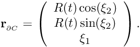can be represented as
${\bf r}_{_{\partial C}} = \left( \begin{array}{c} R(t) \cos(\xi_2) \\ R(t) \sin(\xi_2) \\ \xi_1 \\ \end{array} \right).$
In fluid problems with free surfaces or in fluid-structure interaction (FSI) problems, the domain boundary might have to be determined as part of the solution. In such cases, the boundary will have some computational representation. For instance, in an FSI computation in which a shell structure bounds the fluid domain, each shell finite element defines a small part of the fluid domain boundary and the shell element's local coordinates provide a parametrisation of some part of the boundary in a form similar to the one shown above.

The common feature of these two examples is that, in both cases, the boundary is represented by a parametrised position vector. The GeomObject base class provides an abstract interface for such situations. In its most basic form, a ‘geometric object’ simply provides a parametrisation of its shape by implementing the GeomObject's pure virtual member function

GeomObject::position(xi,r)

which computes the position vector r at the coordinates specified by the vector xi. GeomObject also provides a large number of additional interfaces in the form of (broken) virtual functions. The most important of these is the time-dependent version of the above function

GeomObject::position(xi,t,r)

which computes the position vector r at the coordinates specified by the vector xi at the previous discrete time level t. We follow the usual convention that

for t=0 the vector r is the position vector at the current time, time = Time::time() = Time::time(0)
for t=1 it represents the position at the previous (discrete) time level t, i.e. at the continuous time time = Time::time() - Time::dt() = Time::time(1)
etc.

By default, the virtual member function GeomObject::position(xi,t,r) calls the steady version GeomObject::position(xi,r), so it only needs to be overloaded for genuinely time-dependent geometric objects (by default, the code execution terminates if the time-dependent version is called for ${\tt t} \ne 0;$ the function needs to be overloaded if this is not appropriate).

Further virtual member functions provide interfaces for the determination of the first and second spatial and temporal derivatives of the position vector, allowing the computation of boundary velocities, accelerations and curvatures, etc. These interfaces are provided as broken virtual functions, so they only need to be overloaded if/when the functionality is actually required in a particular application.

Typically, the shape of a GeomObject depends on a certain number of parameters (in the above examples, the radius of the cylinder and the displacements of the shell element, respectively) which can be unknowns in the problem. We therefore store these parameters as (geometric) Data, whose values can be pinned or free.

Domains and Macro Elements

For the purposes of mesh generation, we represent curvilinear domains by objects that are derived from the base class Domain and use GeomObjects to represent the curvilinear boundaries. For instance, the QuarterCircleSectorDomain sketched in the figure below is bounded by the geometric object Ellipse that parametrises the domain's curved boundary, shown in red.

Consider the coarse discretisation of the domain shown in the Fig. (a) and assume that element 2 (a four-node quad element from the QElement family) is scheduled for refinement into four son elements. As discussed above, by default the Nodes of the son elements are established/created as follows:

If a Node already exists in the father element we store the pointer to the existing Node in the son element's Node_pt vector.
If a Node needs to be created, we determine its position from the geometric mapping of the father element. Thus the five new Nodes that need to be created when element 2 is refined, are placed at their father element's (i.e. element 2's) local coordinates (0,0), (0,1), (0,-1), (1,0) and (-1,0). The father element's
RefineableQElement<2>::get_x(...)

determines the nodal position via a call to QElement::interpolated_x(...). Similarly, the nodal values of the new Nodes are determined by using the interpolated values in the father element.

Illustration of mesh refinement with and without macro elements

For the element 0, this procedure would be perfectly adequate, as the domain boundary after refinement would (still) be captured exactly. However, when refining element 2 by this procedure, the new Node on the boundary is positioned on the straight line between the two boundary Nodes in the father element and not on the curved boundary itself, as shown in Fig. (b). Hence repeated mesh refinement will not lead to a better representation of the domain geometry and preclude convergence to the exact solution.

To overcome this problem, objects of type Domain provide a decomposition of the domain into a number of so-called MacroElements, as sketched in Fig. (c). Boundaries of the MacroElements are either given by (parts of) the (exact) curvilinear boundaries (as specified by the Domain's GeomObjects) or by (arbitrary and usually straight) internal edges (or, in 3D, faces). In 2D, MacroElements provide a mapping ${\bf r}(S_0,S_1)$ from a local coordinate system , with $S_i \in [-1..1]^2$ , to the points inside the MacroElement via their member function

MacroElement::macro_map(S,r)

oomph::QuadTreeNames::S

@ S

Definition: quadtree.h:62

The mapping needs to be chosen such that for $S_1\in [-1..1]$ the position vector ${\bf r}(S_0=-1,S_1)$ sweeps along the ‘southern’ edge of the MacroElement, etc.; see Fig. (e). The form of the macro-element mapping is obviously not unique and it depends on the MacroElement's topology. The class QMacroElement<2> provides a mapping that is suitable for 2D quadrilateral elements and can therefore be used with RefineableQElement<2> s.

The constructors for objects of type Domain typically require a vector of pointers to the GeomObjects that define its boundaries. The Domain constructor then usually employs function pointers to the GeomObject::position(...) function to define the MacroElement boundaries. Once built, the MacroElements are accessible via the member function

Domain::macro_element_pt(...).

We illustrate the macro-element based mesh generation and adaptation process for the case of RefineableQuadMesh meshes. Assume that the domain is represented by an object of type Domain. We build a coarse initial mesh which contains as many RefineableQElement<2>s as there are QMacroElements in the Domain. We associate each RefineableQElement<2> with one of the QMacroElements by storing a pointer to the QMacroElement in FiniteElement::Macro_elem_pt. Next, we use the QMacroElements' macro map to determine the RefineableQElement<2>'s nodal positions such that, e.g., the RefineableQElement<2>'s SW node is placed at the QMacroElement 's local coordinates , etc. The fraction of the QMacroElement that is spanned by each RefineableQElement<2> is represented by the maximum and minimum values of the QMacroElement's local coordinates; the RefineableQElement<2> constructor initially sets these values to the defaults of +1.0 and -1.0, respectively, indicating that the RefineableQElement<2> spans the entire area of the corresponding QMacroElement.

With this additional information, we modify the
RefineableQElement<2>::build() process as follows:

After creating the son elements, we set their FiniteElement::Macro_elem_pt to that of their father.
We adjust the son's maximum and minimum MacroElement coordinates so that they span the appropriate fraction of the MacroElement. For instance, for the SW son element of element 2 in the above sketch, we set $S_0^{min}=-1, \ S_0^{max}=0, \ S_1^{min}=-1, \ S_1^{max}=0$ . Should this element get refined again, we set its NW son element's coordinates to $S_0^{min}=-1, \ S_0^{max}=-0.5, \ S_1^{min}=-0.5, \ S_1^{max}=0$ , etc.
The nodal positions of newly created Nodes are determined via calls to the father element's RefineableQElement<2>::get_x(...) function. If the father element is associated with a MacroElement (indicated by a non-NULL RefineableQElement<2>::Macro_elem_pt pointer), this function does not refer to QElement::interpolated_x(...) (i.e. the FE mapping) but places the new Node at the appropriate point inside the father's MacroElement. This ensures that Nodes that are created on the Mesh boundaries get placed on the Domain boundary, as shown in Fig. (d).
In time-dependent, moving mesh problems, the history of the new Nodes' position is established by calls to the time-dependent version of the MacroElement::macro_map(...) function, which in turn refers to the time-dependent GeomObject::position(...) function of the GeomObjects that define the Domain boundaries. Hence for all new Nodes, Node::x(t,i) for t>0, returns the position the Node would have had if it had already existed at the previous time level t.
We retain the original procedure for initialising the current and previous values at the new Nodes and continue to determine them by interpolation from the father element, based on the father element's local coordinates. (We cannot determine the function values at the exact new nodal positions because new Nodes can be located outside their father elements.)

Macro-element-based node updates in moving mesh problems

Once a Mesh is associated with a Domain, the function Mesh::node_update() updates the nodal positions in response to a change in the shape of the GeomObjects that define the Domain boundaries. [Note: This function updates all nodal positions first and then updates the positions of the hanging nodes to subject them to the hanging node constraints.] Alternative procedures for the update of the nodal positions in response to changes in the domain boundary are implemented in the AlgebraicMesh, SpineMesh and SolidMesh classes.

PDF file

A pdf version of this document is available.