This is the final and most complex problem in our series of demo codes for the unsteady heat equation. We re-visit the moving domain problem considered in the previous example and solve it with a combination of spatial and temporal adaptivity.

The two-dimensional unsteady heat equation with flux boundary conditions in a moving domain. Solve

$\sum_{i=1}^2\frac{\partial^2 u}{\partial x_i^2} = \frac{\partial u}{\partial t} + f\left(x_1,x_2,t\right), \ \ \ \ \ \ \ \ \ \ (1)$

in the domain

, bounded by the coordinate axes and the time-dependent ellipse

$\mathbf{r}_{ellipse}(\xi,t) = \left( \begin{array}{c} \big(a+\hat{a}\sin(2\pi t/\hat{T})\big) \cos(\xi) \\ \big(b+\hat{b}\sin(2\pi t/\hat{T})\big) \sin(\xi) \end{array} \right), \ \ \ \ \ \ \ \ \ \ (2)$

subject to Neumann boundary conditions,

$\left. \frac{\partial u}{\partial n}\right|_{\partial D_{Neumann}}= - \left. \frac{\partial u}{\partial x_2}\right|_{\partial D_{Neumann}}= g_0, \ \ \ \ \ \ \ \ \ \ (3)$

along the horizontal domain boundary $\partial D_{Neumann} = \{ (x_1,x_2) | x_1 \in [0,1], x_2=0 \}$ , and to Dirichlet boundary conditions,

$\left. u\right|_{\partial D_{Dirichlet}}=h_0, \ \ \ \ \ \ \ \ \ \ (4)$

elsewhere.

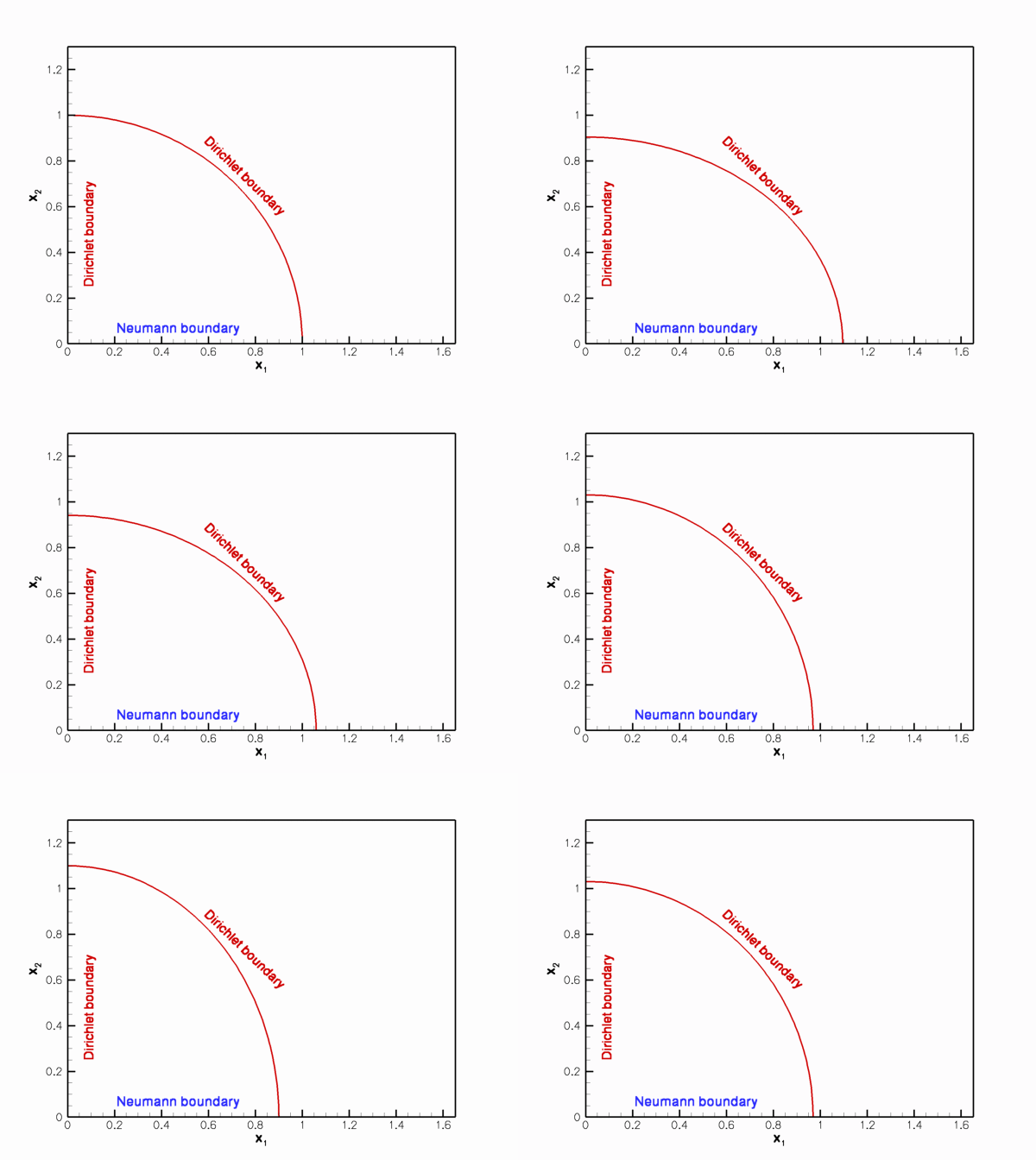
Sketch of the time-dependent domain and the boundary conditions.

The initial conditions are given by

$u(x_1,x_2,t=0)=k_0(x_1,x_2), \ \ \ \ \ \ \ \ \ \ (5)$

where the functions $f, g_0, \ h_0$ and

are given.

We choose the functions $f, g_0, \ h_0$ and so that

$u_0(x_1,x_2,t) = \tanh\bigg[1-\alpha\bigg(\tan\Phi \big(x_1-\beta\tanh[ \gamma\cos\left(2\pi t\right)]\big)- x_2\bigg)\bigg] \ \ \ \ \ \ \ \ \ \ (6)$

is the exact solution.

The solution represents the "usual" tanh profile, whose steepness is controlled by the parameter $\alpha$ so that for $\alpha \gg 1$ the solution approaches a step. The step is oriented at an angle $\Phi$ against the -axis and its position varies periodically. The parameter $\beta$ controls the amplitude of the step's lateral displacement, while $\gamma$ determines the rate at which its position changes. For $\gamma \gg 1$ , the step remains stationary for most of the period and then translates rapidly parallel to the -axis, making this a very challenging problem.

Background: Combined spatial and temporal adaptivity

When solving the above problem with pure spatial adaptivity, we observed that the error of the computed solution increased noticeably during phases when the "step" moved rapidly through the domain, suggesting that the error is due to the temporal rather than the spatial discretisation. If you attempted the exercises suggested at the end of that demo problem, you will have confirmed this by observing that the error is reduced when the time-integration is performed with a smaller timestep. Since the solution only undergoes rapid changes during short periods of time, the use of temporal adaptivity is highly desirable. Before demonstrating that the combined use of temporal and spatial adaptivity only requires trivial changes to the driver code with purely spatial adaptivity, we briefly comment on the strategy employed by oomph-lib's doubly-adaptive unsteady Newton solver

doubly_adaptive_unsteady_newton_solve(dt,epsilon_t,max_adapt,first)

This Newton solver performs the spatial and temporal adaptations sequentially, as follows:

Given a mesh and the solution on that mesh at time , we first advance the solution to time , adjusting the timestep until the global temporal error norm computed by Problem::global_temporal_error_norm() falls below the target error specified by the (double) argument epsilon_t. The (double) argument dt, specifies the suggestion for the timestep.
Once a temporally accurate solution has been computed on that mesh, we perform up to max_adapt spatial adaptations to reduce the spatial error. We re-compute the solution on the adapted meshes, using the (fixed) timestep selected previously by the temporal adaptation. Once the spatial adaptations are complete, we could, in principle, re-evaluate the temporal error and, if required, re-compute the timestep yet again – at a significant additional cost. We omit this further adjustment and accept the solution "as is".

As before, the boolean argument first indicates if the first timestep is being computed (see the
example without temporal adaptivity for more information on this important issue). As in the case of pure temporal adaptivity, the adaptive unsteady Newton solver returns a suggestion for the size of the next timestep.

The implementation

Since the spatial and temporal adaptations are performed independently, adding "double adaptivity" to the existing driver code with pure spatial adaptivity only requires the implementation of the additional member function Problem::global_temporal_error_norm(). In the current problem we can use the one that we created for the example with pure temporal adaptivity. Furthermore, we pass a true boolean flag to the constructor of the BDF<2> timestepper, to make it adaptive. That's all! Apart from a few (optional) improvements to the dump/restart functions (discussed below), the code does not require any other changes.

Some results

The figure below shows a snapshot of the animated solution, obtained from the doubly adaptive simulation.

Snapshot of the solution.

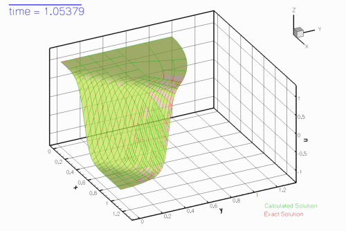
When viewing the animation of the solution, note how the time-bar grows much more rapidly during phases when the solution only changes slowly, reflecting the larger timestep used during these phases.

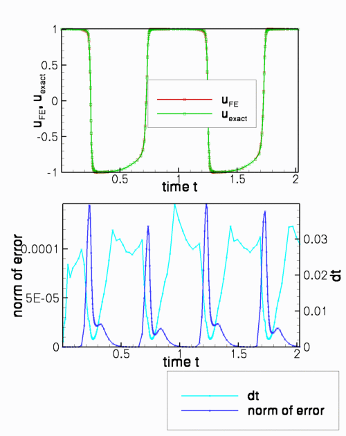
The time-traces shown below compare the exact and computed solutions, and document the variations in timestep and the norm of the error throughout the simulation, for a temporal error target of epsilon_t = $10^{-2}.$ The plots show clearly how the adaptive timestepper selects a much larger timestep during the phases when the solution only changes slowly. However, the error during phases of rapid change is still relatively large – the comparison between the exact and computed solution shows that the two are not graphically indistinguishable. We ought to do better!

Time trace of the solution, the error and the timestep chosen by the adaptive timestepper for a temporal error target of 1E-2.

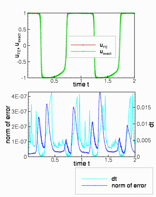
The time-traces below show the results from a second simulation with a smaller target error of epsilon_t = $10^{-3}$ . The exact and computed solutions are now graphically indistinguishable and the error has been reduced significantly – at the cost of having to take much smaller timesteps throughout the simulation. Without adaptive time-stepping, this simulation would become very expensive as timesteps as small as $dt = 2 \times 10^{-4}$ are required to properly resolve the solution during the phases of rapid change.

Time trace of the solution, the error and the timestep chosen by the adaptive timestepper for a temporal error target of 1E-3.

Comments and Exercises

Customising the dump/restart procedure

In two earlier examples, we commented on two undesirable features of the default dump/restart procedures:

The restart files do not record the counter (stored in a DocInfo object) that we typically use to label the output files. Therefore the output files produced in the restarted run start with label "0", making it difficult to merge the data files from the original and restarted simulations.
In an adaptive simulation, the restart files do not record the adaptive timestepper's suggestion for the next timestep, therefore the first timestep in the restarted simulation is performed with the timestep that was used when the solution was dumped to disk, leading to slight differences in the history of the timesteps chosen; see the plot shown at the end of the discussion of the example with purely temporal adaptivity.

To address these problems, we modified the Problem class for the present example slightly: We added the DocInfo object which stores the label for the output file to the Problem's private member data, and provide storage for the size of the next timestep suggested by the adaptive timestepper.

private:
 
 /// Doc info object
 DocInfo Doc_info;
 
 /// Suggestion for next timestep (stored to allow it to be written
 /// to (or read from) restart file)
 double Next_dt;

[We also provide a public access function, double next_dt(), to the suggested next timestep; see Do NOT use public member data in any classes .]

We initialise the output label in the Problem constructor,

//========start_of_constructor============================================
/// Constructor for UnsteadyHeat problem on deformable ellipse domain.
/// Pass pointer to source function.
//========================================================================
template<class ELEMENT>
RefineableUnsteadyHeatProblem<ELEMENT>::RefineableUnsteadyHeatProblem(
 UnsteadyHeatEquations<2>::UnsteadyHeatSourceFctPt source_fct_pt)
 : Source_fct_pt(source_fct_pt)
{
 
 // Setup labels for output
 //------------------------
 
 // Output directory
 Doc_info.set_directory("RESLT");
 
 // Output number
 Doc_info.number()=0; 

and set Next_dt to the initial timestep when the initial condition is assigned in set_initial_condition():

   // Choose initial timestep
   double dt0=0.005;
 
   // Initialise timestep -- also sets the weights for all timesteppers
   // in the problem.
   initialise_dt(dt0);
 
   // Use this as the first "suggested" timestep
   Next_dt=dt0;

We modify the timestepping loop so that the adaptive timestepper's suggestion for the next timestep is stored in the Problem's private data member Next_dt, which is accessible via the public member function next_dt():

 // Timestepping loop
 while (problem.time_pt()->time()<t_max)
  {
   // Take timestep with temporal and spatial adaptivity
   double dt_new=
   problem.doubly_adaptive_unsteady_newton_solve(dt,problem.epsilon_t(),
                                                 max_adapt,first);
   cout << "Suggested new dt: " << dt_new << std::endl;
   dt=dt_new;
   
   // Store for restart
   problem.next_dt()=dt_new;
 
   // Now we've done the first timestep -- don't re-set the IC
   // in subsequent steps
   first=false;
   
   // Reduce the number of spatial adaptations to one per 
   // timestep -- too scared that the interpolation error will 
   // wipe out any further gains...
   max_adapt=1;
   
   //Output solution
   problem.doc_solution();
 
  }

Since the Problem now has access to the DocInfo object (and therefore to the label that we use to identify the output files), and to the suggested next timestep, we write both to the restart file, adding brief comments behind the "raw" data.

//=======start_of_dump_it=================================================
/// Dump the solution to disk
//========================================================================
template<class ELEMENT>
void RefineableUnsteadyHeatProblem<ELEMENT>::dump_it(ofstream& dump_file)
{
 
 // Write step number
 dump_file << Doc_info.number() << " # step number" << std::endl;
 
 // Write suggested next timestep
 dump_file << Next_dt << " # suggested next timestep" << std::endl;
 
 // Dump the refinement pattern and the generic problem data
 Problem::dump(dump_file);
  
} // end of dump_it

These values are then read during the restart:

//=========start_of_restart===============================================
/// Read solution from disk
//========================================================================
template<class ELEMENT>
void RefineableUnsteadyHeatProblem<ELEMENT>::restart(ifstream& restart_file)
{
 // Read line up to termination sign
 string input_string;
 getline(restart_file,input_string,'#');
 
 // Ignore rest of line
 restart_file.ignore(80,'\n');
 
 // Read in step number
 Doc_info.number()=unsigned(atof(input_string.c_str()));
 
 // Increment number for next solution
 Doc_info.number()++;
 
 // Read line up to termination sign
 getline(restart_file,input_string,'#');
 
 // Ignore rest of line
 restart_file.ignore(80,'\n');
 
 // Read suggested next timestep
 Next_dt=double(atof(input_string.c_str()));
 
 // Refine the mesh and read in the generic problem data
 Problem::read(restart_file);
 
} // end of restart

[The slightly clumsy read procedure is required to ensure that the comments that follow the "raw" data are ignored.]

Following the assignment of the initial conditions, the first timestep for the timestepping loop in the main function can now be obtained from next_dt() since Next_dt will either have been set to the actual first timestep used when setting up the initial conditions at time , or to the next timestep that had been suggested by the adaptive timestepper when the restart file was created.

Here are the time-traces for the solution and the timesteps from the original and the restarted simulations – apart from the (very small) roundoff errors due to the finite precision in which all data is recorded in the restart files, they are now in perfect agreement.

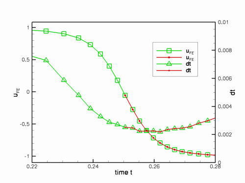
Time-traces of the solution and the timestep for the original (green) and restarted (red) simulations with the customised dump/restart procedure.

Do NOT use public member data in any classes

A little aside: Yes, we really do recommend storing the suggestion for the size of the next timestep as private member data and providing an access function to it. This must seem like (and indeed is) slight overkill in the present context: Why can't we just store it as public member data and avoid having to write the access function? The answer is: Because public data is bad and it's a good habit to avoid it as a matter of principle – even in trivial examples.

Source files for this tutorial

The source files for this tutorial are located in the directory: demo_drivers/unsteady_heat/two_d_unsteady_heat_2adapt/
The driver code is: demo_drivers/unsteady_heat/two_d_unsteady_heat_2adapt/two_d_unsteady_heat_2adapt.cc

PDF file

A pdf version of this document is available.