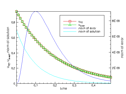
This is our first time-dependent example problem. We will demonstrate that, compared to the solution of steady problems, the solution of time-dependent problems only requires a few additional steps:

The creation of a suitable TimeStepper object and its addition to the Problem's list of timesteppers. (Problems may employ multiple TimeSteppers – a key requirement for the simulation of multiphysics problems.)
The initialisation of the timestep, dt.
Setting the initial conditions by assigning suitable values for the Data objects' "history values" and the Nodes' "positional history values".
Optionally: (Re-)implementing the empty virtual functions Problem::actions_before_implicit_timestep() and Problem::actions_after_implicit_timestep(), e.g. to update time-dependent boundary conditions before each timestep.

Once these steps have been performed, oomph-lib's unsteady Newton solver, Problem::unsteady_newton_solve(...), may be called to advance the solution from its state at time to its new state at $t \ +$ dt.

The example problem

We will illustrate the basic timestepping procedures by considering the solution of the 2D unsteady heat equation in a square domain:

The two-dimensional unsteady heat equation in a square domain. Solve

$\sum_{i=1}^2\frac{\partial^2 u}{\partial x_i^2} = \frac{\partial u}{\partial t} + f\left(x_1,x_2,t\right), \ \ \ \ \ \ \ \ \ \ (1)$

in the square domain $D = \{x_i \in [0,1]; i=1,2 \}$ , subject to the Dirichlet boundary conditions

$\left. u\right|_{\partial D}=g_0 \ \ \ \ \ \ \ \ \ \ (2)$

and initial conditions

$u(x_1,x_2,t=0)=h_0(x_1,x_2), \ \ \ \ \ \ \ \ \ \ (3)$

where the functions

and

are given.

Here we consider the unforced case, , and choose boundary and initial conditions that are consistent with the exact solution

$u_0(x_1,x_2,t) = e^{-Kt}\sin\left( \sqrt{K} \left( x_1 \cos \Phi + x_2 \sin \Phi\right)\right), \ \ \ \ \ \ \ \ \ \ (4)$

where and $\Phi$ are constants, controlling the decay rate of the solution and its spatial orientation, respectively.

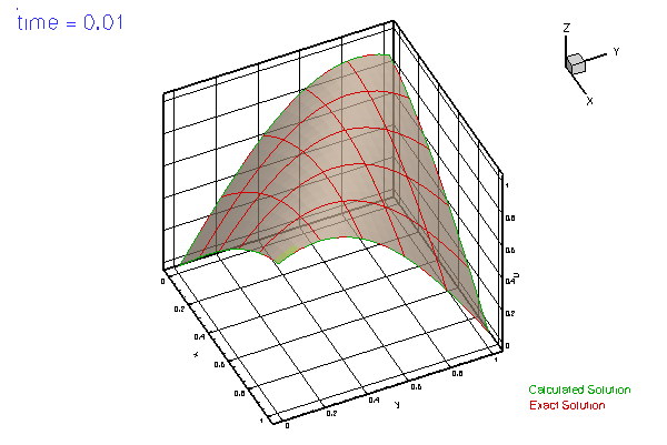
The figure below shows a plot of computed and exact solutions at time (for an animation
click here).

Plot of the exact and computed solutions.

Time evolution of the computed and exact solutions at a control node, the global error norm and the norm of the solution.

Global parameters and functions

As usual, we store the problem parameters in a namespace.

//======start_of_ExactSolnForUnsteadyHeat=====================
/// Namespace for unforced exact solution for UnsteadyHeat equation 
//====================================================================
namespace ExactSolnForUnsteadyHeat
{
 
 /// Decay factor
 double K=10;
 
 /// Angle of bump
 double Phi=1.0; 
 
 /// Exact solution as a Vector
 void get_exact_u(const double& time, const Vector<double>& x, 
                  Vector<double>& u)
 {
  double zeta=cos(Phi)*x[0]+sin(Phi)*x[1];
  u[0]=exp(-K*time)*sin(zeta*sqrt(K));
 }
 
 /// Exact solution as a scalar
 void get_exact_u(const double& time, const Vector<double>& x, double& u)
 {
  double zeta=cos(Phi)*x[0]+sin(Phi)*x[1];
  u=exp(-K*time)*sin(zeta*sqrt(K));
 }
 
 /// Source function to make it an exact solution 
 void get_source(const double& time, const Vector<double>& x, double& source)
 {
  source = 0.0;
 }
 
} // end of ExactSolnForUnsteadyHeat

The driver code

We start by building the Problem object, create a DocInfo object to label the output files, and open a trace file in which we will record the time evolution of the solution and the error. We choose the length t_max of the simulation and the (constant) timestep, dt.

//=======start_of_main====================================================
/// Driver code for unsteady heat equation
//========================================================================
int main()
{
 
 // Build problem
 UnsteadyHeatProblem<QUnsteadyHeatElement<2,4> >
  problem(&ExactSolnForUnsteadyHeat::get_source);
 
 // Setup labels for output
 DocInfo doc_info;
 
 // Output directory
 doc_info.set_directory("RESLT");
 
 // Output number
 doc_info.number()=0;
 
 // Open a trace file
 ofstream trace_file;
 char filename[100];   
 sprintf(filename,"%s/trace.dat",doc_info.directory().c_str());
 trace_file.open(filename);
 trace_file << "VARIABLES=\"time\",\"u<SUB>FE</SUB>\","
            << "\"u<SUB>exact</SUB>\",\"norm of error\",\"norm of solution\""
            << std::endl;
 
 // Choose simulation interval and timestep
 double t_max=0.5;
 double dt=0.01;

Before using any of oomph-lib's timestepping functions, the timestep dt must be passed to the Problem's timestepping routines by calling the function Problem::initialise_dt(...) which sets the weights for all timesteppers in the problem.

Next we assign the initial conditions by calling set_initial_condition(), to be discussed in more detail below, and document the initial conditions.

 // Initialise timestep -- also sets the weights for all timesteppers
 // in the problem.
 problem.initialise_dt(dt);
 
 // Set IC
 problem.set_initial_condition();
 
 //Output initial condition
 problem.doc_solution(doc_info,trace_file);
 
 //Increment counter for solutions 
 doc_info.number()++;

Finally, we execute the timestepping loop and document the computed solutions.

 // Find number of steps
 unsigned nstep = unsigned(t_max/dt);
 
 // Timestepping loop
 for (unsigned istep=0;istep<nstep;istep++)
  {
   cout << " Timestep " << istep << std::endl;
   
   // Take timestep
   problem.unsteady_newton_solve(dt);
   
   //Output solution
   problem.doc_solution(doc_info,trace_file);
   
   //Increment counter for solutions 
   doc_info.number()++;
  }
 
 // Close trace file
 trace_file.close();
 
 
}; // end of main

In this loop, each call to the unsteady Newton solver, Problem::unsteady_newton_solve(...), advances the solution from its current state, at time Problem::time_pt()->time(), to $t \ +$ dt. The unsteady Newton solver automatically "shifts" the history values "backwards" and advances the value of the continuous time.

The problem class

The Problem classes for time-dependent problems are very similar to those for steady problems. The most important additional member functions are Problem::actions_before_implicit_timestep() and Problem::actions_after_implicit_timestep() (both defined as empty virtual functions in the Problem base class) and set_initial_condition(). The functions Problem::actions_before_implicit_timestep() and Problem::actions_after_implicit_timestep() are called automatically by oomph-lib's unsteady Newton solver Problem::unsteady_newton_solve() and may be used to update any time-dependent boundary conditions before the Newton solve, or to perform any postprocessing steps after a timestep has been completed. Here we only use the first of these two functions.

We note that the (self-explanatory) function set_initial_condition() overwrites an empty virtual function in the Problem base class. While the assignment of initial conditions could, in principle, be performed by any other function, e.g. the Problem constructor, we strongly recommend using this function to facilitate the extension to spatial adaptivity. (In spatially adaptive computations of time-dependent problems, a standard interface for the re-assignment of initial conditions following mesh adaptations is required; we will discuss this aspect in
another example).

Finally, the private member data Control_node_pt provides storage for a pointer to a control Node at which we shall document the evolution of the solution.

//=====start_of_problem_class=========================================
/// UnsteadyHeat problem 
//====================================================================
template<class ELEMENT>
class UnsteadyHeatProblem : public Problem
{
 
public:
 
 /// Constructor
 UnsteadyHeatProblem(UnsteadyHeatEquations<2>::UnsteadyHeatSourceFctPt 
 source_fct_pt);
 
 /// Destructor (empty)
 ~UnsteadyHeatProblem(){}
 
 /// Update the problem specs after solve (empty)
 void actions_after_newton_solve() {}
 
 /// Update the problem specs before solve (empty)
 void actions_before_newton_solve() {}
 
 /// Update the problem specs after solve (empty)
 void actions_after_implicit_timestep() {}
 
 /// Update the problem specs before next timestep: 
 /// Set Dirchlet boundary conditions from exact solution.
 void actions_before_implicit_timestep();
 
 /// Set initial condition (incl previous timesteps) according
 /// to specified function. 
 void set_initial_condition();
 
 /// Doc the solution
 void doc_solution(DocInfo& doc_info, ofstream& trace_file);
 
private:
 
 /// Pointer to source function
 UnsteadyHeatEquations<2>::UnsteadyHeatSourceFctPt Source_fct_pt;
 
 /// Pointer to control node at which the solution is documented
 Node* Control_node_pt;
 
}; // end of problem class

The problem constructor

We start by constructing the TimeStepper, the second-order accurate BDF<2> timestepper from the BDF family, and pass a pointer to it to the Problem, using the member function Problem::add_time_stepper_pt(...). As the name of this function indicates, oomph-lib can operate with multiple timesteppers – an essential feature in multi-physics problems. (For instance, in fluid-structure interaction-problems timestepping for the solid equations might be performed with a timestepper from the Newmark family, while a BDF timestepper might be used for the Navier–Stokes equations.) When called for the first time, the function
Problem::add_time_stepper_pt(...) creates the Problem's Time object (accessible via Problem::time_pt()) with sufficient storage for the history of previous timesteps. This is required if the timestep is adjusted during the simulation, e.g. when an adaptive timestepper is used. (If further TimeSteppers which require more storage are added subsequently, Problem::add_time_stepper(...) updates the amount of storage in the Problem's Time object accordingly).

//========start_of_constructor============================================
/// Constructor for UnsteadyHeat problem in square domain
//========================================================================
template<class ELEMENT>
UnsteadyHeatProblem<ELEMENT>::UnsteadyHeatProblem(
 UnsteadyHeatEquations<2>::UnsteadyHeatSourceFctPt source_fct_pt) : 
 Source_fct_pt(source_fct_pt)
{ 
 
 // Allocate the timestepper -- this constructs the Problem's 
 // time object with a sufficient amount of storage to store the
 // previous timsteps. 
 add_time_stepper_pt(new BDF<2>);

Next we set the problem parameters and build the mesh, passing the pointer to the TimeStepper as the last argument to the mesh constructor.

 // Setup parameters for exact solution
 // -----------------------------------
 
 // Decay parameter
 ExactSolnForUnsteadyHeat::K=5.0;
 
 // Setup mesh
 //-----------
 
 // Number of elements in x and y directions
 unsigned nx=5;
 unsigned ny=5;
 
 // Lengths in x and y directions
 double lx=1.0;
 double ly=1.0;
 
 // Build mesh
 mesh_pt() = new RectangularQuadMesh<ELEMENT>(nx,ny,lx,ly,time_stepper_pt());

The position of the pointer to the timestepper in the list of arguments to the mesh constructor reflects another oomph-lib convention:

A general convention

Recall that all Data objects store a pointer to a TimeStepper that translates their "history values" into approximations of the values' time derivatives. The required number of "history values" depends on the specific timestepper. For instance, a BDF<1> timestepper (the backward Euler scheme) requires storage of the solution at the previous timestep; the BDF<2> timestepper computes an approximation of the time-derivative, based on the solution at two previous timesteps, etc.

Nodes (which are Data!) are typically built by the Mesh constructor using the FiniteElement's member function FiniteElement::construct_node(...). This function takes a pointer to the timestepper from which the required amount of storage for the "history values" is extracted. To facilitate the (re-)use of meshes in steady and time-dependent problems, we adopt the convention that

The final argument of all mesh constructors should be the pointer to a TimeStepper which defaults to &Mesh::Default_TimeStepper – a (static) instantiation of oomph-lib's dummy steady timestepper, Steady.

This convention allows the use of meshes in steady problems without having to (artificially) create a timestepper. The following code fragment illustrates the implementation of this approach in a mesh constructor:

//=======================================================================
/// Some mesh class
//=======================================================================
template <class ELEMENT>
class SomeMesh : public virtual Mesh
{
 
public:
 
  /// \short Constructor: Pass number of elements and pointer to timestepper.
  /// Note that the timestepper defaults to the Steady default timestepper.
  SomeMesh(const unsigned& n_element, TimeStepper* time_stepper_pt=
           &Mesh::Default_TimeStepper)
   {
   
     [...]
 
 
     // Allocate storage for all n_element elements in the mesh
     Element_pt.resize(n_element); 
 
     // Create first element and store it (in its incarnation as        
     // a GeneralisedElement) in the Mesh's Element_pt[] array
     Element_pt[0] = new ELEMENT;
 
     // Create the element's first node and store it in the
     // Mesh's Node_pt[] array. [The member function
     // Mesh::finite_element_pt(...) recasts the pointer to the
     // GeneralisedElement to a pointer to a FiniteElement -- only      
     // FiniteElements have a member function construct_node(...)]
     Node_pt[0] = finite_element_pt(0)->construct_node(0,time_stepper_pt);
 
     [...]
 
   }
 
[...]
 
};

Next, we apply the boundary conditions, pinning the values at all boundary nodes.

 // Set the boundary conditions for this problem: 
 // ---------------------------------------------
 // All nodes are free by default -- just pin the ones that have 
 // Dirichlet conditions here. 
 unsigned n_bound = mesh_pt()->nboundary();
 for(unsigned b=0;b<n_bound;b++)
  {
   unsigned n_node = mesh_pt()->nboundary_node(b);
   for (unsigned n=0;n<n_node;n++)
    {
     mesh_pt()->boundary_node_pt(b,n)->pin(0); 
    }
  } // end of set boundary conditions

Finally, we loop over the elements and pass the pointer to the source function.

 // Complete the build of all elements so they are fully functional
 //----------------------------------------------------------------
 
 // Find number of elements in mesh
 unsigned n_element = mesh_pt()->nelement();
 
 // Loop over the elements to set up element-specific 
 // things that cannot be handled by constructor
 for(unsigned i=0;i<n_element;i++)
  {
   // Upcast from FiniteElement to the present element
   ELEMENT *el_pt = dynamic_cast<ELEMENT*>(mesh_pt()->element_pt(i));
 
   //Set the source function pointer
   el_pt->source_fct_pt() = Source_fct_pt;
  }
 
 // Do equation numbering
 cout <<"Number of equations: " << assign_eqn_numbers() << std::endl; 
 
} // end of constructor

Actions before (implicit) timestep

We overload the (empty) virtual function Problem::actions_before_implicit_timestep() to update the time-dependent boundary conditions (2), using the current value of the continuous time from the Problem's Time object.

//=========start of actions_before_implicit_timestep===============================
/// Actions before timestep: update the domain, then reset the 
/// boundary conditions for the current time.
//========================================================================
template<class ELEMENT>
void UnsteadyHeatProblem<ELEMENT>::actions_before_implicit_timestep()
{
 // Get current time
 double time=time_pt()->time();
 
 //Loop over the boundaries
 unsigned num_bound = mesh_pt()->nboundary();
 for(unsigned ibound=0;ibound<num_bound;ibound++)
  {
   // Loop over the nodes on boundary
   unsigned num_nod=mesh_pt()->nboundary_node(ibound);
   for (unsigned inod=0;inod<num_nod;inod++)
    {
     Node* nod_pt=mesh_pt()->boundary_node_pt(ibound,inod);
     double u;
     Vector<double> x(2);
     x[0]=nod_pt->x(0);
     x[1]=nod_pt->x(1);
     // Get current values of the boundary conditions from the
     // exact solution
     ExactSolnForUnsteadyHeat::get_exact_u(time,x,u);
     nod_pt->set_value(0,u);
    }
  }
} // end of actions_before_implicit_timestep

Set initial condition

Before starting a time-dependent simulation, the current and history values of all Data objects must be initialised. In a BDF timestepping scheme, the history values represent the solution at previous discrete timesteps. In the present problem (where the exact solution is known – admittedly, a somewhat artificial situation) we can therefore assign the history values by looping over the previous timesteps and setting the history values with Data::set_value(...).

Important: oomph-lib's UnsteadyHeatEquations are based on the Arbitrary-Lagrangian-Eulerian (ALE) formulation of the unsteady heat equation to permit computations in moving domains; we will illustrate this capability in
another example. In such problems, the nodal positions may vary as a function of time. In the present problem, the computation is performed in a fixed domain, therefore we initialise the previous nodal positions with their current values, accessed via the member function Node::x(t,i) which returns (a reference to) the i -th nodal coordinate at previous timestep t.

A general convention

Many functions in oomph-lib have steady and time-dependent versions which usually differ in their first argument. Typically, the first argument of the time-dependent function is an additional (unsigned) integer, t, say. As a general convention, the time-dependent versions return values (or perform actions) that are appropriate for the current time if called with t=0, and return values (or perform actions) that are appropriate for previous time levels if the argument is set to t>0. Note that we refer to previous time levels, rather than previous timesteps, because history values do not necessarily represent values at previous timesteps, as they do for BDF schemes. For instance, in Newmark timestepping schemes, the history values include approximations of the first and second time-derivatives at the previous timestep.

Another general convention

While, in general, not all "history values" represent the solution at previous timesteps, the "history values" that do, should be (and, for any existing TimeSteppers, are) listed before those that represent other quantities. The number of history values required/used by a TimeStepper may be obtained from its member function

TimeStepper::nprev_values()

As an example, BDF<4>::nprev_values() returns 4. The total number of history values (including the current value!) is returned by

TimeStepper::ntstorage()

As an example, BDF<4>::ntstorage() returns 5.

Here is the source code for the set_initial_condition() function:

//======================start_of_set_initial_condition====================
/// Set initial condition: Assign previous and current values
/// from exact solution.
//========================================================================
template<class ELEMENT>
void UnsteadyHeatProblem<ELEMENT>::set_initial_condition()
{ 
 // Backup time in global Time object
 double backed_up_time=time_pt()->time();
         
 // Past history needs to be established for t=time0-deltat, ...
 // Then provide current values (at t=time0) which will also form
 // the initial guess for the first solve at t=time0+deltat
 
 // Vector of exact solution value
 Vector<double> soln(1);
 Vector<double> x(2);
 
 //Find number of nodes in mesh
 unsigned num_nod = mesh_pt()->nnode();
 
 // Set continuous times at previous timesteps:
 // How many previous timesteps does the timestepper use?
 int nprev_steps=time_stepper_pt()->nprev_values();
 Vector<double> prev_time(nprev_steps+1);
 for (int t=nprev_steps;t>=0;t--)
  {
   prev_time[t]=time_pt()->time(unsigned(t));
  } 
 
 // Loop over current & previous timesteps
 for (int t=nprev_steps;t>=0;t--)
  {
   // Continuous time
   double time=prev_time[t];
   cout << "setting IC at time =" << time << std::endl;
   
   // Loop over the nodes to set initial guess everywhere
   for (unsigned n=0;n<num_nod;n++)
    {
     // Get nodal coordinates
     x[0]=mesh_pt()->node_pt(n)->x(0);
     x[1]=mesh_pt()->node_pt(n)->x(1);
 
     // Get exact solution at previous time
     ExactSolnForUnsteadyHeat::get_exact_u(time,x,soln);
     
     // Assign solution
     mesh_pt()->node_pt(n)->set_value(t,0,soln[0]);
     
     // Loop over coordinate directions: Mesh doesn't move, so 
     // previous position = present position
     for (unsigned i=0;i<2;i++)
      {
       mesh_pt()->node_pt(n)->x(t,i)=x[i];
      }
    } 
  }
 
 // Reset backed up time for global timestepper
 time_pt()->time()=backed_up_time;
 
} // end of set_initial_condition

Post-processing

As in many previous examples, this member function outputs the computed solution, the exact solution and the error. We augment the solution data by tecplot text and geometries to facilitate the visualisation and record the time evolution of the solution and the error in the trace file.

//=======start_of_doc_solution============================================
/// Doc the solution
//========================================================================
template<class ELEMENT>
void UnsteadyHeatProblem<ELEMENT>::
doc_solution(DocInfo& doc_info,ofstream& trace_file)
{ 
 ofstream some_file;
 char filename[100];
 
 // Number of plot points
 unsigned npts;
 npts=5;
 
 
 cout << std::endl;
 cout << "=================================================" << std::endl;
 cout << "Docing solution for t=" << time_pt()->time() << std::endl;
 cout << "=================================================" << std::endl;
 
 
 // Output solution 
 //-----------------
 sprintf(filename,"%s/soln%i.dat",doc_info.directory().c_str(),
         doc_info.number());
 some_file.open(filename);
 mesh_pt()->output(some_file,npts);
 
 // Write file as a tecplot text object
 some_file << "TEXT X=2.5,Y=93.6,F=HELV,HU=POINT,C=BLUE,H=26,T=\"time = " 
           << time_pt()->time() << "\"";
 // ...and draw a horizontal line whose length is proportional
 // to the elapsed time
 some_file << "GEOMETRY X=2.5,Y=98,T=LINE,C=BLUE,LT=0.4" << std::endl;
 some_file << "1" << std::endl;
 some_file << "2" << std::endl;
 some_file << " 0 0" << std::endl;
 some_file << time_pt()->time()*20.0 << " 0" << std::endl;
 some_file.close();
 
 
 // Output exact solution 
 //----------------------
 sprintf(filename,"%s/exact_soln%i.dat",doc_info.directory().c_str(),
         doc_info.number());
 some_file.open(filename);
 mesh_pt()->output_fct(some_file,npts,time_pt()->time(),
                       ExactSolnForUnsteadyHeat::get_exact_u); 
 some_file.close();
 
 // Doc error
 //----------
 double error,norm;
 sprintf(filename,"%s/error%i.dat",doc_info.directory().c_str(),
         doc_info.number());
 some_file.open(filename);
 mesh_pt()->compute_error(some_file,
                          ExactSolnForUnsteadyHeat::get_exact_u,
                          time_pt()->time(),
                          error,norm); 
 some_file.close();
 
 // Doc solution and error
 //-----------------------
 cout << "error: " << error << std::endl; 
 cout << "norm : " << norm << std::endl << std::endl;
 
 // Get exact solution at control node
 Vector<double> x_ctrl(2);
 x_ctrl[0]=Control_node_pt->x(0);
 x_ctrl[1]=Control_node_pt->x(1);
 double u_exact;
 ExactSolnForUnsteadyHeat::get_exact_u(time_pt()->time(),x_ctrl,u_exact);
 trace_file << time_pt()->time() << " " 
            << Control_node_pt->value(0) << " " 
            << u_exact << " " 
            << error   << " " 
            << norm    << std::endl;
 
} // end of doc_solution

Comments and Exercises

The current example only illustrates the most basic timestepping procedures. In subsequent examples we will demonstrate oomph-lib's
dump and restart functions, the use of adaptive timestepping, the use of spatial adaptivity, computations in moving domains, and the combination of temporal and spatial adaptivity.

We stress that setting the initial conditions in a "real" problem often presents a delicate step, especially if higher-order timesteppers from the BDF family are used. This is because in the absence of a known exact solution, the initial condition (3) only provides enough information to determine a single "history value" at each node – the value at the initial time. oomph-lib's timestepping procedures provide several functions that allow the simulation to be initiated with an "impulsive start", corresponding to a past history in which the boundary condition (3) describes the system's state for all $t \le 0$ rather than only at . For instance, the top-level function Problem::assign_initial_values_impulsive() sets the "history values" of all Data objects and the Nodes' "positional history values" to values that are appropriate for an impulsive start from the currently assigned nodal values and positions. The following exercises aim to explore this functionality.

Exercises

Replace the call to problem.set_initial_condition() in the main function by a call to Problem::assign_initial_values_impulsive() and analyse the results. [Hint: When Data objects are created, their values are initialised to zero.]
Confirm that the loop over the coordinate directions
// Loop over coordinate directions: Mesh doesn't move, so

// previous position = present position

for (unsigned i=0;i<2;i++)

{

mesh_pt()->node_pt(n)->x(t,i)=x[i];

}

in set_initial_condition(), can be replaced by
time_stepper_pt()->assign_initial_positions_impulsive(

mesh_pt()->node_pt(n));

[This statement could then be moved outside the loop over the previous time levels.]
Confirm that the initialisation of the previous nodal positions is essential by commenting out this step – see the
ALE example for further details on computations in moving domains.
Overwrite the correct assignment of the "history values" in set_initial_condition() by adding the statement Problem::assign_initial_values_impulsive() at the end of this function (rather than bypassing the assignment completely as in the first exercise). Repeat this with the BDF<1> and BDF<4> timesteppers and explain the different behaviour.
Examine the accuracy of the various BDF timesteppers by re-running the simulations with various timesteppers and with different timesteps.

Source files for this tutorial

The source files for this tutorial are located in the directory: demo_drivers/unsteady_heat/two_d_unsteady_heat/
The driver code is: demo_drivers/unsteady_heat/two_d_unsteady_heat/two_d_unsteady_heat.cc

PDF file

A pdf version of this document is available.