Simulations of time-dependent problem can be very time consuming and it is important to be able to restart simulations, e.g. to continue a run after a system crash, etc. We shall illustrate oomph-lib's dump/restart capabilities by re-visiting the 2D unsteady heat equation discussed in a previous example.

The two-dimensional unsteady heat equation in a square domain. Solve

$\sum_{i=1}^2\frac{\partial^2 u}{\partial x_i^2} = \frac{\partial u}{\partial t} + f\left(x_1,x_2,t\right), \ \ \ \ \ \ \ \ \ \ (1)$

in the square domain $D = \{x_i \in [0,1]; i=1,2 \}$ , subject to the Dirichlet boundary conditions

$\left. u\right|_{\partial D}=g_0 \ \ \ \ \ \ \ \ \ \ (2)$

and initial conditions

$u(x_1,x_2,t=0)=h_0(x_1,x_2), \ \ \ \ \ \ \ \ \ \ (3)$

where the functions

and

are given.

As before, we consider the unforced case, , and choose boundary and initial conditions that are consistent with the exact solution

$u_0(x_1,x_2,t) = e^{-Kt}\sin\left( \sqrt{K} \left( x_1 \cos \Phi + x_2 \sin \Phi\right)\right), \ \ \ \ \ \ \ \ \ \ (4)$

where and $\Phi$ are constants, controlling the decay rate of the solution and its spatial orientation, respectively.

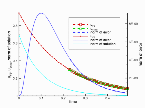
The figure below shows a plot of computed and exact solution at a control node as a function of time. The solid lines represent quantities computed during the original simulation; the dashed line shows the corresponding data from a second simulation that was restarted with the restart file generated at timestep 23 of the original simulation.

Time evolution of the computed and exact solutions at a control node, the global error norm and the norm of the solution. Solid lines: original simulation; dashed lines: restarted simulation.

Most of the driver code for this example is identical to that discussed in the previous example, therefore we only discuss the modifications required to enable the dump and restart operations:

We use optional command line arguments to specify the name of the restart file. If the code is run without any command line arguments, we start the simulation at time and generate the initial conditions as in the previous example
We add dump and restart functions to the Problem class and call the dump function when post-processing the solution in doc_solution(...).
We modify the Problem member function set_initial_condition()
so that the initial conditions are read from the restart file if a restart file was specified on the command line.

Global parameters and functions

The namespace ExactSolnForUnsteadyHeat that stores the problem parameters is identical to that in the previous example.

The driver code

The only change to the main function is that we record the command line arguments and store them in the namespace CommandLineArgs

//=======start_of_main====================================================
/// Driver code for unsteady heat equation with option for
/// restart from disk: Only a single command line argument is allowed.
/// If specified it is interpreted as the name of the restart file.
//========================================================================
int main(int argc, char* argv[])
{
 
 // Store command line arguments
 CommandLineArgs::setup(argc,argv);

The rest of the main function is identical to that in the previous example.

The problem class

The problem class contains the two additional member functions

 /// Dump problem to disk to allow for restart.
 void dump_it(ofstream& dump_file);
 
 /// Read problem for restart from specified restart file.
 void restart(ifstream& restart_file);

The problem constructor

The problem constructor is identical to that in the previous example.

The problem destructor

The problem destructor is identical to that in the previous example.

Actions before timestep

This function is identical to that in the previous example.

Set initial condition

We start by checking the validity of the command line arguments, accessible via the namespace CommandLineArgs, as only a single command line argument is allowed. If a command line argument is provided, it is interpreted as the name of the restart file. We try to open the file and, if successful, pass the input stream to the restart(...) function, discussed below. If no command line arguments are specified, we generate the initial conditions, essentially as in the
previous example. The only difference is that in the current version of the code, we moved the specification and initialisation of the timestep from the main function into set_initial_condition(). This is because in a restarted simulation, the value of dt must be consistent with that used in the original simulation. If the simulation is restarted, the generic Problem::read(...) function, called by restart(...), automatically initialises the previous timestep; otherwise we have to perform the initialisation ourselves.

//======================start_of_set_initial_condition====================
/// Set initial condition: Assign previous and current values
/// from exact solution or from restart file.
//========================================================================
template<class ELEMENT>
void UnsteadyHeatProblem<ELEMENT>::set_initial_condition()
{ 
 
 // Pointer to restart file
 ifstream* restart_file_pt=0;
 
 // Restart?
 //---------
 // Restart file specified via command line [all programs have at least
 // a single command line argument: their name. Ignore this here.]
 if (CommandLineArgs::Argc==1)
  {
   cout << "No restart -- setting IC from exact solution" << std::endl;
  }
 else if (CommandLineArgs::Argc==2)
  {
   // Open restart file
   restart_file_pt= new ifstream(CommandLineArgs::Argv[1],ios_base::in);
   if (restart_file_pt!=0)
    {
     cout << "Have opened " << CommandLineArgs::Argv[1] << 
      " for restart. " << std::endl;
    }
   else
    {
     std::ostringstream error_stream;
     error_stream 
      << "ERROR while trying to open " << CommandLineArgs::Argv[1] << 
      " for restart." << std::endl;
 
     throw OomphLibError(
      error_stream.str(),
      OOMPH_CURRENT_FUNCTION,
      OOMPH_EXCEPTION_LOCATION);
    }
  }
 // More than one command line argument?
 else 
  {
   std::ostringstream error_stream;
   error_stream << "Can only specify one input file\n" 
                << "You specified the following command line arguments:\n";
   //Fix this
   CommandLineArgs::output();
 
   throw OomphLibError( 
    error_stream.str(),
    OOMPH_CURRENT_FUNCTION,
    OOMPH_EXCEPTION_LOCATION);
  }
 
 
 // Read restart data:
 //-------------------
 if (restart_file_pt!=0)
  {
 
   // Read the problem data from the restart file
   restart(*restart_file_pt);
 
  }
 // Assign initial condition from exact solution
 //---------------------------------------------
 else
  {
   
   // Choose timestep
   double dt=0.01;
   
   // Initialise timestep -- also sets the weights for all timesteppers
   // in the problem.
   initialise_dt(dt);
   
   // Backup time in global Time object
   double backed_up_time=time_pt()->time();
   
   // Past history fo needs to be established for t=time0-deltat, ...
   // Then provide current values (at t=time0) which will also form
   // the initial guess for the first solve at t=time0+deltat
   
   // Vector of exact solution value
   Vector<double> soln(1);
   Vector<double> x(2);
   
   //Find number of nodes in mesh
   unsigned num_nod = mesh_pt()->nnode();
   
   // Set continuous times at previous timesteps
   int nprev_steps=time_stepper_pt()->nprev_values();
   Vector<double> prev_time(nprev_steps+1);
   for (int itime=nprev_steps;itime>=0;itime--)
    {
     prev_time[itime]=time_pt()->time(unsigned(itime));
    } 
   
   // Loop over current & previous timesteps
   for (int itime=nprev_steps;itime>=0;itime--)
    {
     // Continuous time
     double time=prev_time[itime];
     cout << "setting IC at time =" << time << std::endl;
     
     // Loop over the nodes to set initial guess everywhere
     for (unsigned n=0;n<num_nod;n++)
      {
       // Get nodal coordinates
       x[0]=mesh_pt()->node_pt(n)->x(0);
       x[1]=mesh_pt()->node_pt(n)->x(1);
       
       // Get intial solution
       ExactSolnForUnsteadyHeat::get_exact_u(time,x,soln);
       
       // Assign solution
       mesh_pt()->node_pt(n)->set_value(itime,0,soln[0]);
       
       // Loop over coordinate directions: Previous position = present position
       for (unsigned i=0;i<2;i++)
        {
         mesh_pt()->node_pt(n)->x(itime,i)=x[i];
        }
      } 
    }
   
   // Reset backed up time for global timestepper
   time_pt()->time()=backed_up_time;
 
  }
 
 
} // end of set_initial_condition

Post-processing

The Problem member function doc_solution(...) is identical to that in the previous example, apart from the addition of a call to the new dump_it(...) function, discussed below.

 // Write restart file
 sprintf(filename,"%s/restart%i.dat",doc_info.directory().c_str(),
         doc_info.number());
 some_file.open(filename);
 dump_it(some_file);
 some_file.close();

Dumping the solution

The Problem::dump(...) function writes the generic Problem data in ASCII format to the specified output file. The content of the file can therefore be inspected and, if necessary, manipulated before a restart. However, the specific content of the file is generally of little interest – it is written in a format that can be read by the corresponding function Problem::read(...).

Briefly, the dump file contains:

A flag that indicates if the data was produced by a time-dependent simulation.
The current value of the "continuous" time, i.e. the value returned by Problem::time_pt()->time();
The number of previous timesteps, dt, stored in the Problem's Time object, and their values.
The values and history values for all Data objects in the Problem, as well as the present and previous coordinates of all Nodes.

The "raw data" is augmented by brief comments that facilitate the identification of individual entries.

In the present problem, the generic Problem::dump(...) function is sufficient to record the current state of the simulation, therefore no additional information needs to be added to the dump file. The section Comments and Exercises below contains an exercise that illustrates how to customise the dump function to record additional parameters; the demo code with spatial adaptivity provides another example of a customised dump/restart function.

//=====start_of_dump_it===================================================
/// Dump the solution to disk to allow for restart
//========================================================================
template<class ELEMENT>
void UnsteadyHeatProblem<ELEMENT>::dump_it(ofstream& dump_file)
{
 
 // Call generic dump()
 Problem::dump(dump_file); 
 
} // end of dump_it

Reading a solution from disk

Since the restart file was written by the generic Problem::dump(...) function, it can be read back with the generic Problem::read(...) function. If any additional data had been recorded in the restart file, additional read statements could be added here; see Comments and Exercises.

//=================start_of_restart=======================================
/// Read solution from disk for restart
//========================================================================
template<class ELEMENT>
void UnsteadyHeatProblem<ELEMENT>::restart(ifstream& restart_file)
{
 
 // Read the generic problem data from restart file
 Problem::read(restart_file);
 
} // end of restart

Comments and Exercises

The Problem::dump(...) and Problem::read(...) functions write/read the generic data that is common to all oomph-lib problems. Occasionally, it is necessary to record additional data to re-create the system's state when the simulations is restarted. We will explore this in more detail in another example. Here we provide a brief exercise that illustrates the general idea and addresses a shortcoming of the driver code: Currently the program computes the same number of timesteps, regardless of whether or not the simulation was restarted. If a simulation is restarted, the computation therefore continues past $t=t_{max}.$

Exercises

Change the for loop over the fixed number of timesteps in the main function to a while loop that checks if the continuous time, accessible via Problem::time_pt()->time(), has reached or exceeded $t_{max}$ . This works because the Problem::dump(...) and Problem::read(...) functions dump and restore the value of the continuous time.
Following this trivial change, the restarted simulation is terminated at the appropriate point but the numbering of the output files begins at 0, making it difficult to merge the results from the original and the restarted simulations. Modify the functions dump_it(...) and restart(...) so that they write/read the current label for the output files to/from the restart file.

Hints: (i) You can write to/read from the restart file before calling Problem::dump(...) and Problem::read(...); just make sure you do it in the same order in both functions. (ii) The easiest way to make the label, currently stored in the DocInfo object in the main function, accessible to all member functions in the Problem is to make the DocInfo object a private data member of the Problem class.

Source files for this tutorial

The source files for this tutorial are located in the directory: demo_drivers/unsteady_heat/two_d_unsteady_heat/
The driver code is: demo_drivers/unsteady_heat/two_d_unsteady_heat/two_d_unsteady_heat_restarted.cc

PDF file

A pdf version of this document is available.