In this tutorial we re-visit the solution of fluid-structure interaction problems with (pseudo-)solid fluid mesh updates, focusing on the efficient solution of the governing equations by GMRES, using the problem-specific block-preconditioner developed in

Muddle, R.L., Mihajlovic, M. & Heil, M. (2012) An efficient preconditioner for monolithically-coupled large-displacement fluid-structure interaction problems with pseudo-solid mesh updates. Journal of Computational Physics 231, 7315-7334. DOI: 10.1016/j.jcp.2012.07.001

where full details of the analysis and further results from a variety of other test problems can be found.

Background: Problem formulation, the resulting linear system and the preconditioner

We will demonstrate the development and application of the preconditioner using the problem of flow in a 2D channel with an elastic leaflet discussed in another tutorial and illustrated in the sketch below:

Sketch of the problem.

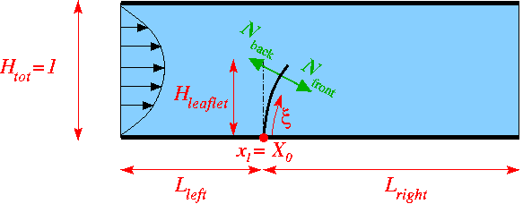
Flow is driven (via an imposed parabolic inflow profile) through a 2D channel which is partially obstructed by a thin-walled elastic leaflet. The fluid leaves the domain at the far downstream end of the channel where we assume parallel, axially traction-free outflow.

We use the same discretisation (2D quadrilateral Taylor-Hood elements for the fluid; 1D Hermite beam elements for the leaflet) as in the original tutorial. However, here we perform the fluid mesh update in response to the deformation of the elastic leaflet using a pseudo-elastic approach. This is done by "wrapping" the underlying QTaylorHoodElement into a PseudoSolidNodeUpdateElement and employing ImposeDisplacementByLagrangeMultiplierElements to impose the deformation of the elastic leaflet onto the (pseudo-solid) fluid mesh. The following tutorials discuss the relevant methodologies:

The discretised problem contains the following types of discrete unknowns:

The fluid degrees of freedom (velocities and pressures).
The nodal positions (real and generalised; the latter representing derivative degrees of freedom in the Hermite elements used to discretise the leaflet; see the beam theory tutorial for details) of the elastic leaflet.
The nodal positions in the fluid mesh.
The nodal values representing the components of the (vector-valued) Lagrange multipliers which impose the motion of the elastic leaflet on the pseudo-elastic fluid mesh. These unknowns only exist for the fluid nodes on the FSI boundary.

Using this classification of the unknowns, the linear system to be solved in the course of the Newton iteration can be re-ordered into the following block structure:

$J_{\rm FSI} \ \Delta {\bf x} = \left[ \begin{array}{c|c|cc} F& &C_{\rm fx}&\\ \hline C_{\rm sf}&S&C_{\rm sx}&\\ \hline &&E&C_{\rm xl}\\ &C_{\rm ls}&C_{\rm lx}&\\ \end{array} \right] \left[ \begin{array}{c} \Delta {\bf F}\\ \hline \Delta {\bf S}\\ \hline \Delta {\bf X}\\ \Delta {\bf L}\\ \end{array} \right] =- \left[ \begin{array}{c} {\bf r}_{\rm f}\\ \hline {\bf r}_{\rm s}\\ \hline {\bf r}_{\rm x}\\ {\bf r}_{\rm l}\\ \end{array} \right] \ \ \ \ \ \ \ \ (1)$

where the vector ${\bf F}$ contains the Navier-Stokes (fluid) unknowns (velocities and pressure), ${\bf S}$ represents unknowns describing the deformation of the fluid-loaded solid, ${\bf X}$ represents the nodal positions in the fluid mesh, and ${\bf L}$ contains the discrete Lagrange multipliers which impose the deformation of the FSI boundary in the fluid mesh. The three diagonal blocks in the Jacobian matrix, $J_{\rm FSI}$ , are the two `‘single-physics’' Jacobian matrices ( , the Navier-Stokes Jacobian; , the tangent stiffness matrix of the fluid-loaded solid) and the Jacobian,

$J_{\rm PS} = \left[ \begin{array}{cc} E&C_{\rm xl}\\ C_{\rm lx}&\\ \end{array} \right]$

associated with the Lagrange-multiplier-constrained pseudo-elasticity problem governing the fluid mesh update, discussed in more detail in another tutorial. The non-zero off-diagonal blocks arise through the interactions between the various single-physics problems: $C_{\rm fx}$ represents the effect of the pseudo-solid unknowns (the nodal positions in the fluid mesh) on the discretised Navier–Stokes equations – this incorporates the so-called shape-derivatives and the time-discretised version of the no-slip condition on the FSI boundary which expresses the fluid velocities in terms of the nodal velocities of the fluid mesh. $C_{\rm sf}$ captures the effect of the fluid traction (pressure and shear stresses) on the fluid-loaded solid. Since the shear stresses depend on gradients of the fluid velocity, the traction is also affected by the nodal positions in the fluid mesh – this dependency gives rise to the matrix $C_{\rm sx}$ . Finally, $C_{\rm ls}$ arises because the prescribed boundary displacement of the fluid mesh depends on the displacement field in the fluid-loaded solid. The zero block reflects the fact that the discretised Navier-Stokes equations do not depend directly on the displacement field of the actual solid. The zero block indicates that the pseudo-solid equations are not affected by the fluid unknowns. The block is zero because the real solid affects the pseudo-solid only indirectly via the Lagrange multiplier constraint (which gives rise to $C_{\rm ls}$ ). Finally, the non-zero blocks in the last block column reflect the fact that the Lagrange multiplier is only used to enforce the displacement constraint in a one-way coupling in which the real solid affects the pseudo-solid but not vice versa. See Muddle, Mihajlovic & Heil (2012) for more detail.

To construct a preconditioner for the linear system (1) we replace the bottom-right $2 \times 2$ block in the Jacobian with the pseudo-solid preconditioner,

${\cal P}_{\rm PS} = \left[ \begin{array}{cc} E_{\rm aug}&\\ &W \end{array} \right] \ \ \ \ \ \ \ \ \ \ \ \ \ \ (2)$

which we discussed in another tutorial. This yields the pseudo-solid FSI preconditioner

${\cal P}_{\rm FSI}=\left[ \begin{array}{c|c|cc} F& &C_{\rm fx}&\\ \hline C_{\rm sf}&S&C_{\rm sx}&\\ \hline &&E_{\rm aug}&\\ &C_{\rm ls}&&W \end{array} \right]. \ \ \ \ \ \ (3)$

The preconditioner can be shown to have a block triangular structure. Its application therefore requires the solution of four subsidiary linear systems involving the matrices , , $E_{\rm aug}$ and and four sparse matrix-vector products with the interaction matrices $C_{\rm fx}$ , $C_{\rm sx}$ , $C_{\rm sf}$ and $C_{ls}$ .

Numerical experiments in Muddle, Mihajlovic & Heil (2012) show that an efficient implementation of the preconditioner is obtained by

replacing the solution of the linear system involving ${\cal P}_{\rm PS}$ by the approximation $\widetilde{\cal P}_{\rm PS}$ discussed in another tutorial,
replacing the solution of the linear system involving the Navier-Stokes Jacobian by an application of Elman, Silvester and Wathen's Least-Squares Commutator (LSC) preconditioner,

and by replacing the remaining block-solves within these preconditioners by a small number of AMG cycles or CG iterations. We retain SuperLU as the (exact) direct solver for the linear system involving the real solid's tangent stiffness matrix .

With these approximations, the computational cost of one application of the preconditioner is linear in the number of unknowns (see Comments and Exercises for a more detailed discussion of this issue). The optimality of the preconditioner can therefore be assessed by demonstrating that the number of GMRES iterations remains constant under mesh refinement.

Implementation and use of the preconditioner

The preconditioner described above is implemented within oomph-lib's (parallel) block preconditioning framework which is described in another tutorial. For the purpose of the implementation, we decompose the preconditioning matrix into the 3x3 main blocks indicated by the vertical and horizontal lines in (1) and (3).

The degrees of freedom within these sub-blocks are classified into "dof-types" on an element-by-element basis, using the functions

GeneralisedElement::ndof_types(...) which returns the number of dof types classified by that element.
GeneralisedElement::get_block_numbers_for_unknowns(...) which associates each degree of freedom (identified by its global equation number) with the dof type within its block.

The default implementation of these functions within the Navier-Stokes elements (which differentiate between the fluid velocity components and the pressure) and the beam elements (which do not distinguish between the different types of degree of freedom) is appropriate for the use with the (subsidiary) preconditioners employed here. The degrees of freedom representing the nodal positions in the (pseudo-solid) fluid mesh need to be sub-divided into those that are and are not constrained by the Lagrange multipliers that impose the deformation of the FSI boundary. This is most conveniently done by overloading the relevant functions in a templated wrapper element, PseudoElasticBulkElement<...>,
as discussed in another tutorial.

Results

We examine the performance of the preconditioner in steady and unsteady test problems. First we perform a sequence of steady solves, incrementing the Reynolds number in steps of 25. The final steady solution is then used as the initial condition for an unsteady simulation in which the inflow is subjected to a time-periodic oscillation. The tables below show the GMRES iteration counts (averaged over all linear solves performed in the course of all Newton iterations) as a function of the mesh refinement (represented by the total number of unknowns) for different implementations of the preconditioner.

Average GMRES iteration counts (steady runs)

`n_dof`	9570	38724	87462	155784
GMRES (blocks solved by SuperLU)	5.88889	5.88889	5.88889	6.11111
GMRES (LSC; blocks solved by SuperLU)	27.8889	36.1111	42.3333	47.2222
GMRES (LSC; pseudo-solid; blocks solved by Hypre/CG)	37.3333	43.2222	49.3333	55.3333

Average GMRES iteration counts (unsteady runs)

`n_dof`	9570	38724	87462	155784
GMRES (blocks solved by SuperLU)	6.5124	6.95868	7.15323	7.2619
GMRES (LSC; blocks solved by SuperLU)	15	15.9256	16.2097	16.6429
GMRES (LSC; pseudo-solid; blocks solved by Hypre/CG)	22.2066	25.3967	27.0484	27.9921

As expected from the theory (see Muddle, Mihajlovic & Heil (2012)), the GMRES iteration counts are small and virtually mesh independent for the exact implementation of the preconditioner. Replacing the (costly) exact solves by (faster) approximate solves leads to a modest increase in the (absolute) number of GMRES iterations. The most significant deterioration of the iteration counts results from the use of the LSC Navier Stokes preconditioner as the inexact solver (subsidiary preconditioner) for the Navier-Stokes block. The behaviour observed here (slight mesh dependence for steady solves; virtual mesh independence (once the mesh is sufficiently fine) for unsteady solves) mirrors that observed in single-physics Navier-Stokes problems.

The benefit of switching to the approximate solves becomes apparent in the next two tables which shows the average cpu times required for the solution of the linear systems by GMRES. (For comparison the times labelled as "SuperLU" show the times when the linear systems (1) are solved directly by SuperLU rather than by GMRES; they illustrate how quickly direct solvers become uncompetitive.) For sufficiently fine discretisations the larger number of GMRES iterations for the inexact solves is more than compensated for by the much lower cost of the preconditioning operations. The final implementation yields cpu times that (at least for unsteady problems) are proportional to the number of unknowns – the hallmark of an optimal solver.

Average linear solver times (steady runs; sec)

`n_dof`	9570	38724	87462	155784
SuperLU	2.71863	33.7939	129.248	325.384
GMRES (blocks solved by SuperLU)	2.31567	15.1042	58.5491	147.531
GMRES (LSC; blocks solved by SuperLU)	2.8051	18.3197	58.7335	138.558
GMRES (LSC; pseudo-solid; blocks solved by Hypre/CG)	3.47733	15.1812	37.6856	73.0526

Average linear solver times (unsteady runs; sec)

`n_dof`	9570	38724	87462	155784
SuperLU	2.06807	25.7064	99.7166	248.082
GMRES (blocks solved by SuperLU)	1.73668	11.1679	42.2051	105.97
GMRES (LSC; blocks solved by SuperLU)	1.87403	11.0113	34.2697	81.4382
GMRES (LSC; pseudo-solid; blocks solved by Hypre/CG)	2.26537	9.40194	22.5644	41.8251

Modifications to the driver code

Most of the driver code is unchanged from the implementation discussed in the original tutorial. We therefore only discuss the modifications required

to perform the fluid mesh update using (pseudo-)elasticity,

and

to employ preconditioned GMRES as the linear solver in the Newton method.

Fluid-mesh udate by pseudo-elasticity

To perform the node update in the fluid mesh in response to the deformation of the leaflet using the equations of large-displacement elasticity we "wrap" the Navier-Stokes element in the doubly-templated PseudoSolidNodeUpdateElement<WRAPPED_ELEMENT, SOLID_ELEMENT> class. The first template argument of this class, WRAPPED_ELEMENT, specifies the type of the "wrapped" element – here the nine-node, 2D quadrilateral QTaylorHoodElement<2>. The second template argument, SOLID_ELEMENT, specifies the SolidElement used to perform the node update – here the nine-node, 2D quadrilateral QPVDElement<2,3>. Since the preconditioner requires the (re-)classification of the pseudo-solid degrees of freedom into constrained and unconstrained nodal positions, we wrap this element too, using the PseudoElasticBulkElement already discussed in another tutorial. The full specification of the fluid element is therefore given by

PseudoSolidNodeUpdateElement<QTaylorHoodElement<2>,

PseudoElasticBulkElement<QPVDElement<2,3> > >

Modifications to the main code

The main code only requires minor changes, all associated with the specification of different solver options. Since we provide the option to use Hypre and Trilinos solvers, we need to activate MPI if oomph-lib has been compiled with MPI support (even if the code is run in serial):

//=======start_of_main=====================================================
/// Driver code 
//=========================================================================
int main(int argc, char **argv)
{
#ifdef OOMPH_HAS_MPI
 MPI_Helpers::init(argc,argv);
#endif

Next we define and process the possible command line flags which are used to select solver options and to specify the spatial resolution

 // Store command line arguments
 CommandLineArgs::setup(argc,argv);
 
 // Multiplier for number of elements in coordinate directions.
 // Used for uniform mesh refinement studies.
 unsigned mesh_multiplier = 2; 
 CommandLineArgs::specify_command_line_flag("--mesh_multiplier",
                                            &mesh_multiplier);
 
 // Suppress use of LSC preconditioner for Navier Stokes block
 CommandLineArgs::specify_command_line_flag("--suppress_lsc");
 
 // Use direct solver (SuperLU)
 CommandLineArgs::specify_command_line_flag("--use_direct_solver");
 
 // Use SuperLU for all block solves
 CommandLineArgs::specify_command_line_flag("--superlu_for_blocks");
 
 // Validation only?
 CommandLineArgs::specify_command_line_flag("--validate");

We then assign the command line flags that were specified and document the ones that were recognised, before building the problem, specifying the heavily wrapped version of the Navier-Stokes element as the template parameter.

 // Parse command line
 CommandLineArgs::parse_and_assign(); 
 
 // Doc what has actually been specified on the command line
 CommandLineArgs::doc_specified_flags();
 
 //Set up the problem
 FSIChannelWithLeafletProblem<PseudoSolidNodeUpdateElement
                              <QTaylorHoodElement<2>,
                               PseudoElasticBulkElement<QPVDElement<2,3> > > >* 
  problem_pt = new  
  FSIChannelWithLeafletProblem<PseudoSolidNodeUpdateElement
                               <QTaylorHoodElement<2>,
                                PseudoElasticBulkElement<QPVDElement<2,3> > > >
  (mesh_multiplier);

The rest of the main code is very similar to the original version discussed in another tutorial and is therefore omitted here.

Choosing the iterative solver and preconditioner

We provide a new function, set_iterative_solver() to switch the solver to GMRES and to instantiate the FSI preconditioner. We start by creating the GMRES solver, using Trilinos' implementation if it is available:

//===========start_iterative_solver=========================================
/// Set iterative solver 
//==========================================================================
template<class ELEMENT>
void FSIChannelWithLeafletProblem<ELEMENT>::set_iterative_solver()
{
 // Create the linear solver
 IterativeLinearSolver* solver_pt=0;
 
 // If we have trilinos, use it
#ifdef OOMPH_HAS_TRILINOS
 
 // Create solver
 solver_pt = new TrilinosAztecOOSolver;
 
 // Use GMRES
 dynamic_cast<TrilinosAztecOOSolver*>(solver_pt)->solver_type() 
  = TrilinosAztecOOSolver::GMRES;
 
#else
 
 // Use oomph-lib's own GMRES
 solver_pt = new GMRES<CRDoubleMatrix>;
 
#endif
 
 // Set solver
 linear_solver_pt() = solver_pt;

Next, we create an instance of the FSI preconditioner for a 2D problem and pass it to the solver:

  
 // Create preconditioner for 2D problem
 unsigned dim=2;
 PseudoElasticFSIPreconditioner* prec_pt=
  new PseudoElasticFSIPreconditioner(dim, this);
 
 // Set preconditioner
 solver_pt->preconditioner_pt() = prec_pt;

The classification of the degrees of freedom within the block preconditioning framework requires the specification of the (pseudo-solid) fluid mesh, the "real" solid mesh and the mesh containing the Lagrange multiplier elements that impose the deformation of the FSI boundary in the fluid mesh:

 // Specify meshes that contain elements which classify the various
 // degrees of freedom:
 prec_pt->set_fluid_and_pseudo_elastic_mesh_pt(Bulk_mesh_pt);
 prec_pt->set_solid_mesh_pt(Wall_mesh_pt);
 prec_pt->set_lagrange_multiplier_mesh_pt(Lagrange_multiplier_mesh_pt);

We provide the option to bypass the use of the LSC Schur complement preconditioner as the subsidiary preconditioner (inexact solver) for the Navier-Stokes block:

 // Use oomph-lib's Schur complement preconditioner as Navier-Stokes
 // subsidiary preconditioner
 if (!CommandLineArgs::command_line_flag_has_been_set("--suppress_lsc"))
  {
   oomph_info << "Enabling LSC preconditioner\n";
   prec_pt->enable_navier_stokes_schur_complement_preconditioner();
  }
 else
  {
   prec_pt->disable_navier_stokes_schur_complement_preconditioner();
   oomph_info << "Not using LSC preconditioner\n";
  } // done disable lsc

By default the preconditioner performs the preconditioning operations as described above, using SuperLU for the block solves in (3). It is possible to specify alternative (approximate) solvers for these. For instance, the behaviour of the LSC preconditioner can be modified by following the pointer to the Schur complement preconditioner

 
 
 // Use approximate block solves?
 //------------------------------
 if (CommandLineArgs::command_line_flag_has_been_set("--superlu_for_blocks"))
  {
   oomph_info << "Use SuperLU for block solves\n";
  }
 else
  {
   oomph_info << "Use optimal block solves\n";
 
   // Get pointer to Navier-Stokes Schur complement preconditioner
   NavierStokesSchurComplementPreconditioner* ns_prec_pt = 
    prec_pt->navier_stokes_schur_complement_preconditioner_pt();

whose behaviour can be modified as discussed in LSC preconditioner tutorial. For instance, to use a block-triangular approximation for the Navier-Stokes momentum block we specify

 
   // Navier Stokes momentum block
   //-----------------------------
 
   // Block triangular for momentum block in LSC precond
   BlockTriangularPreconditioner<CRDoubleMatrix>*
    f_prec_pt = new BlockTriangularPreconditioner<CRDoubleMatrix>;
 
   // Set it
   ns_prec_pt->set_f_preconditioner(f_prec_pt);  

If Hypre is available, we can then (approximately) solve the diagonal blocks using a small number of AMG V-cycles (with settings specified in the helper function LSC_Preconditioner_Helper::set_hypre_preconditioner):

   
#ifdef OOMPH_HAS_HYPRE
 
   // Use Hypre for diagonal blocks
   f_prec_pt->set_subsidiary_preconditioner_function
    (LSC_Preconditioner_Helper::set_hypre_preconditioner);

Similarly, we can use Hypre (with settings appropriate for a 2D Poisson problem) to approximately solve the pressure Poisson systems in the computations of the Schur complement approximation:

 
 
   // Navier Stokes Schur complement/pressure block
   //----------------------------------------------
 
   // Build/set Hypre for Schur complement (pressure) block
   HyprePreconditioner* p_prec_pt = new HyprePreconditioner;
   p_prec_pt->disable_doc_time();   
   Hypre_default_settings::set_defaults_for_2D_poisson_problem(p_prec_pt);   
   ns_prec_pt->set_p_preconditioner(p_prec_pt); 
 
#endif

Approximate solvers for the diagonal blocks in the preconditioner (2) for the the Lagrange-multiplier constrained pseudo-elastic equations can be chosen as discussed in another tutorial. For instance, we can employ a block-upper triangular approximation for the augmented pseudo-elastic block $E_{\rm aug}$ :

 
   // Pseudo elastic block
   //---------------------
 
   // Use block upper triangular preconditioner for (pseudo-)elastic block
   prec_pt->pseudo_elastic_preconditioner_pt()->elastic_preconditioner_type()
    = PseudoElasticPreconditioner::Block_upper_triangular_preconditioner;

Its diagonal blocks can then again be solved by Hypre,

 
#ifdef OOMPH_HAS_HYPRE
 
   // Use Hypre for diagonal blocks of (pseudo-)elastic preconditioner
   prec_pt->pseudo_elastic_preconditioner_pt()->
    set_elastic_subsidiary_preconditioner(
     Pseudo_Elastic_Preconditioner_Subsidiary_Operator_Helper::
     get_elastic_preconditioner_hypre);
 
#endif

Similarly, the linear systems involving the mass matrices in can be solved using diagonally preconditioned CG:

   
#ifdef OOMPH_HAS_TRILINOS
 
   // Use Trilinos CG as subsidiary preconditioner (inexact solver) for
   // linear (sub-)systems to be solved in the Lagrange multiplier block
   prec_pt->pseudo_elastic_preconditioner_pt()->
    set_lagrange_multiplier_subsidiary_preconditioner
    (Pseudo_Elastic_Preconditioner_Subsidiary_Operator_Helper::
     get_lagrange_multiplier_preconditioner);
 
#endif
  }
 
} //end set_iterative_solver

Comments and Exercises

Comments

Further details of the theory, such as the proof of the optimality of the preconditioner, can be found in Muddle, Mihajlovic & Heil (2012).
Note that we retained SuperLU as the solver for the linear system involving the tangent stiffness matrix of the actual, fluid-load solid. In the present example this still leads to an optimal solver since the leaflet is modelled as a 1D beam structure whose number of unknowns increases much more slowly than the number of unknowns in the fluid mesh when the meshes are refined uniformly. If the solid is modelled as a "proper" solid, the use of a direct solver for the solution of the linear systems involving becomes sub-optimal. The member function
PseudoElasticFSIPreconditioner::set_solid_preconditioner(...)

can then be used to specify a subsidiary preconditioner (inexact solver) for the linear systems involving .

Exercises

Experiment with different preconditioner settings and explore the performance of the preconditioner at different Reynolds numbers. The script run.sh used to generate the data presented above, may be helpful.

Source files for this tutorial

The source files for this tutorial are located in the directory:

demo_drivers/interaction/pseudo_solid_fsi_channel_with_leaflet
The driver code is:

demo_drivers/interaction/pseudo_solid_fsi_channel_with_leaflet/fsi_channel_with_leaflet_precond.cc

PDF file

A pdf version of this document is available.