In this example we consider the flow in a 2D channel which is partially obstructed by an oscillating leaflet. We consider the case where the motion of the leaflet is prescribed – this is a "warm-up exercise" for the corresponding FSI problem in which the leaflet is an elastic structure.

The Problem

The figure below shows a sketch of the problem: A 2D channel of height $H^*_{tot}$ and length $L^*_{left} + L^*_{right}$ is partially occluded by a (zero-thickness) leaflet of height $H^*_{leaflet}$ . The leaflet is parametrised by a Lagrangian coordinate $\xi^*$ so that the position vector to a material point on the leaflet is given by ${\bf R}^*_w(\xi^*,t^*)$ , and we assume that the leaflet performs time-periodic oscillations with period Steady Poiseuille flow with average velocity is imposed at the left end of the channel while we assume that the outflow is parallel and axially traction-free.

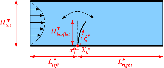
Sketch of the problem in dimensional

We non-dimensionalise all length and coordinates on the channel width, $H^*_{tot}$ , time on the natural timescale of the flow, $H^*_{tot}/U^*$ , the velocities on the mean velocity, , and the pressure on the viscous scale. The problem is then governed by the non-dimensional Navier-Stokes equations

$Re \left( St \frac{\partial u_i}{\partial t} + u_j \frac{\partial u_i}{\partial x_j} \right) = - \frac{\partial p}{\partial x_i} + \frac{\partial }{\partial x_j} \left[ \left( \frac{\partial u_i}{\partial x_j} + \frac{\partial u_j}{\partial x_i} \right) \right],$

where $Re = \rho U^* H_0^* / \mu$ and , and

$\frac{\partial u_i}{\partial x_i} = 0,$

subject to parabolic inflow

${\bf u} = 6 x_2 (1-x_2) {\bf e}_1$

at the inflow cross-section; parallel, axially-traction-free outflow at the outlet; and no-slip on the stationary channel walls, ${\bf u} = {\bf 0}$ . The no-slip condition on the leaflet is

${\bf u} = \frac{\partial {\bf R}_w(\xi,t)}{\partial t}$

and the leaflet performs oscillations with non-dimensional period $T = T^* U^* / H^*_{tot}$ . Here is a sketch of the non-dimensional version of the problem:

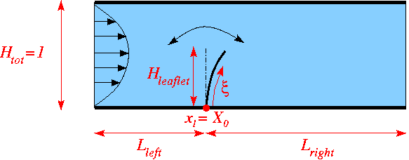
Sketch of the problem in dimensionless variables.

An interesting feature of this problem is that even though the leaflet is assumed to have negligible thickness its presence will generate a pressure jump between its two faces. (The velocities are continuous because the no-slip condition imposes the same velocity on both faces.) When discretising the problem with QTaylorHood elements (for which the pressure varies continuously across the element boundaries), the mesh must therefore be "opened up" with a cut along the position of the leaflet. This is done in the constructor of the ChannelWithLeafletMesh which forms the basis of RefineableAlgebraicChannelWithLeafletMesh used to discretise this problem. (See Further comments and exercises for a more detailed discussion of the mesh.)

Results

The figure below shows a snapshot of the flow field
(pressure contours and instantaneous streamlines) for a Reynolds number of and an oscillation period of , as well as the corresponding fluid mesh. Note how oomph-lib's automatic mesh adaptation has refined the mesh near the tip of the leaflet where the pressure has a singularity.

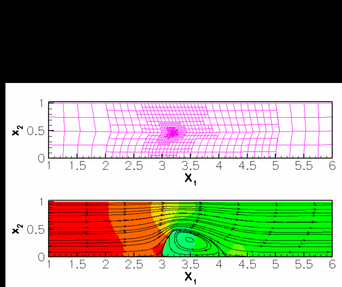
Mesh (top) and flow field (bottom).

The corresponding animation illustrates the algebraic node update strategy (implemented with an AlgebraicMesh, discussed in more detail in another tutorial) and the evolution of the flow field. Note that the instantaneous streamlines intersect the (impermeable) leaflet because the leaflet is not stationary.

The global parameters

As usual we use a namespace to define the (single) global parameter, the Reynolds number.

//==start_of_global_parameters=======================================
/// Global parameters
//===================================================================
namespace Global_Physical_Variables
{
 
 /// Reynolds number
 double Re=20.0;
 
} // end_of_namespace

Specification of the leaflet geometry

We specify the leaflet geometry and its time-dependent motion by representing it as a GeomObject. The GeomObject has one Lagrangian and two Eulerian coordinates, and its geometry is characterised by its length, the x-coordinate of its origin, , and the period and amplitude of the horizontal and vertical tip deflection.

//===start_of_leaflet_class===========================================
/// GeomObject representing a vertical leaflet that performs
/// bending and stretching oscillations. 
//====================================================================
class Leaflet : public GeomObject
{
 
public:
 
 /// Constructor: Pass length (in Lagrangian coordinates),
 /// the amplitude of the horizontal and vertical deflection of the tip,
 /// the x-coordinate of the origin and the period of the oscillation.
 /// Passes the number of Lagrangian and Eulerian coordinates to the
 /// constructor of the GeomObject base class.
 Leaflet(const double& length, const double& d_x,const double& d_y,
         const double& x_0, const double& period, Time* time_pt)
  : GeomObject(1,2), Length(length), D_x(d_x), D_y(d_y), X_0(x_0),
   T(period),Time_pt(time_pt) {}
 
 
 /// Destructor -- emtpy
 virtual ~Leaflet(){}
 
 /// Position vector, r, to the point identified by  
 /// its 1D Lagrangian coordinate, xi (passed as a 1D Vector) at discrete time
 /// level t (t=0: present; t>0: previous).
 void position(const unsigned& t, const Vector<double>& xi, 
               Vector<double>& r) const
  {
    using namespace MathematicalConstants;
 
   //Position
    r[0] =  X_0 + D_x*xi[0]*xi[0]/Length/Length*sin(2.0*Pi*Time_pt->time(t)/T);
    r[1] = xi[0]*(1.0+D_y/Length*0.5*(1.0-cos(4.0*Pi*Time_pt->time(t)/T)));
  }
 
 /// Steady version: Get current shape
 void position(const Vector<double>& xi, Vector<double>& r) const
  {
   position(0,xi,r); 
  }
 
 /// Number of geometric Data in GeomObject: None.
 unsigned ngeom_data() const {return 0;}  
 
 /// Length of the leaflet
 double length() { return Length; }
 
 /// Amplitude of horizontal tip displacement
 double& d_x() {return D_x;}
 
 /// Amplitude of vertical tip displacement
 double d_y() {return D_y;}
 
 /// x-coordinate of leaflet origin
 double x_0() {return X_0;}
 
private :
 
 /// Length in terms of Lagrangian coordinates
 double Length;
 
 /// Horizontal displacement of tip
 double D_x;
 
 /// Vertical displacement of tip
 double D_y;
 
/// Origin
 double X_0;
 
 /// Period of the oscillations
 double T;
 
 /// Pointer to the global time object
 Time* Time_pt;
 
}; //end_of_the_GeomObject

The driver code

We store the command line arguments, create a DocInfo object, and assign the parameters that specify the domain and the leaflet geometry:

//======start_of_main==================================================
/// Driver code -- pass a command line argument if you want to run
/// the code in validation mode where it only performs a few steps
//=====================================================================
int main(int argc, char* argv[])
{
 
 // Store command line arguments
 CommandLineArgs::setup(argc,argv);
 
 // Set up doc info
 DocInfo doc_info; 
 doc_info.set_directory("RESLT");
 doc_info.number()=0;
 
 // Parameters for the leaflet
 //----------------------------
 
 // Height
 double h_leaflet = 0.5;
 
 
 // Tip deflection
 double d_x = 0.25;
 double d_y = -0.05;
 
 // x-positon of root
 double x_0 = 3.0; 
 
 // Period of the oscillation on the natural timescale of the flow
 double period = 20.0;
 
 
 //Parameters for the domain
 //-------------------------
 
 // Length of the mesh to right and left of the leaflet
 double l_left =2.0;
 double l_right= 3.0;
 
 // Total height of domain (unity because lengths have been scaled on it)
 double h_tot=1.0;
 
 // Initial number of element rows/columns in various mesh regions
 unsigned nleft=8;
 unsigned nright=12;
 unsigned ny1=2;
 unsigned ny2=2; 

Next we build the problem and assign the time-stepping parameters (as usual, fewer timesteps are used during a validation run which is identified by a non-zero number of command line arguments):

 
 //Build the problem
 ChannelWithLeafletProblem<AlgebraicElement<RefineableQTaylorHoodElement<2> > >
  problem(l_left, l_right, h_leaflet,
          h_tot,nleft, nright,ny1,ny2,
          d_x, d_y, x_0,
          period);
 
 
 // Number of timesteps per period
 unsigned nsteps_per_period=40;
 
 // Number of periods
 unsigned nperiod=3; 
 
 // Number of timesteps (reduced for validation)
 unsigned nstep=nsteps_per_period*nperiod;
 if (CommandLineArgs::Argc>1)
  {
   nstep=3;
  }
 
 //Timestep: 
 double dt=period/double(nsteps_per_period);
 
 /// Initialise timestep 
 problem.initialise_dt(dt);

We start the simulation with a steady solve, allowing up to five levels of adaptive refinement (fewer if we are performing a validation run):

 
 
 /// Set max. number of adaptations (reduced for validation)
 unsigned max_adapt=5;
 if (CommandLineArgs::Argc>1)
  {
   max_adapt=2;
  }
 
 // Do steady solve first -- this also sets the history values
 // to those corresponding to an impulsive start from the
 // steady solution
 problem.steady_newton_solve(max_adapt);
 
 /// Output steady solution
 problem.doc_solution(doc_info);
 doc_info.number()++;

Finally, we enter the proper timestepping loop, allowing one spatial adaptation per timestep and suppressing the re-assignment of initial conditions following an adaptation by setting the parameter first to false (see the discussion of timestepping with automatic mesh adaptation in another tutorial.)

 
 
 /// Reduce the max number of adaptations for time-dependent simulation
 max_adapt=1;
 
 // We don't want to re-assign the initial condition 
 bool first=false;
 
// Timestepping loop
 for (unsigned istep=0;istep<nstep;istep++)
  { 
   // Solve the problem
   problem.unsteady_newton_solve(dt,max_adapt,first);
   
   // Output the solution
   problem.doc_solution(doc_info);
   
   // Step number
   doc_info.number()++;
 
  }
 
 
}//end of main

The Problem class

The problem class has the usual member functions to perform actions after the mesh adaptation and before every implicit timestep:

//==start_of_problem_class===========================================
/// Problem class
//===================================================================
template<class ELEMENT>
class ChannelWithLeafletProblem : public Problem
{
 
public:
 
 /// Constructor: Pass the length of the domain at the left
 /// of the leaflet lleft,the length of the domain at the right of the
 /// leaflet lright,the height of the leaflet hleaflet, the total height
 /// of the domain htot, the number of macro-elements at the left of the
 /// leaflet nleft, the number of macro-elements at the right of the
 /// leaflet nright, the number of macro-elements under hleaflet ny1,
 /// the number of macro-elements above hleaflet ny2,the x-displacement
 /// of the leaflet d_x,the y-displacement of the leaflet d_y,the abscissa 
 /// of the origin of the leaflet x_0, the period of the moving leaflet.
 ChannelWithLeafletProblem(const double& l_left,
                           const double& l_right, const double& h_leaflet,
                           const double& h_tot,
                           const unsigned& nleft, const unsigned& nright,
                           const unsigned& ny1, const unsigned&  ny2,
                           const double& d_x,const double& d_y,
                           const double& x_0, const double& period);  
 
 /// Destructor (empty)
 ~ChannelWithLeafletProblem(){}
 
 /// Overloaded access function to specific mesh
 RefineableAlgebraicChannelWithLeafletMesh<ELEMENT>* mesh_pt() 
  {
   // Upcast from pointer to the Mesh base class to the specific 
   // element type that we're using here.
   return dynamic_cast<RefineableAlgebraicChannelWithLeafletMesh<ELEMENT>*>(
    Problem::mesh_pt());
  }
 
 /// Update after solve (empty)
 void actions_after_newton_solve(){}
 
 /// Update before solve (empty)
 void actions_before_newton_solve(){}
 
 /// Actions after adaptation: Pin redundant pressure dofs
 void actions_after_adapt();
 
 /// Update the velocity boundary condition on the moving leaflet
 void actions_before_implicit_timestep();
 
 /// Doc the solution
 void doc_solution(DocInfo& doc_info);
 
private:
 
 /// Pointer to the GeomObject
 GeomObject* Leaflet_pt;
 
};

The problem constructor

We construct the timestepper and the GeomObject that represents the leaflet, and pass it pointers to them to the constructor of the RefineableAlgebraicChannelWithLeafletMesh (discussed in more detail in Further comments and exercises).

 
 
 
 
//==start_of_constructor=================================================
/// Constructor
//=======================================================================
template <class ELEMENT>
ChannelWithLeafletProblem<ELEMENT>::ChannelWithLeafletProblem(
 const double& l_left,
 const double& l_right, const double& h_leaflet,
 const double& h_tot,
 const unsigned& nleft, const unsigned& nright,
 const unsigned& ny1, const unsigned&  ny2,
 const double& d_x,const double& d_y,
 const double& x_0, const double& period)
{
 // Allocate the timestepper
 add_time_stepper_pt(new BDF<2>);
 
 //Create the geometric object that represents the leaflet
 Leaflet_pt = new Leaflet(h_leaflet, d_x, d_y, x_0, period, time_pt()) ;
 
//Build the mesh
Problem::mesh_pt()=new RefineableAlgebraicChannelWithLeafletMesh<ELEMENT>(
 Leaflet_pt,
 l_left, l_right,
 h_leaflet,
 h_tot,nleft,
 nright,ny1,ny2,
 time_stepper_pt());     

Next we create the spatial error estimator and loop over the elements to set the pointers to the relevant physical parameters.

 
 
 // Set error estimator
 Z2ErrorEstimator* error_estimator_pt=new Z2ErrorEstimator;
 dynamic_cast<RefineableAlgebraicChannelWithLeafletMesh<ELEMENT>*>(mesh_pt())->
  spatial_error_estimator_pt()=error_estimator_pt;
 
 
 // Loop over the elements to set up element-specific 
 // things that cannot be handled by constructor
 unsigned n_element = mesh_pt()->nelement();
 for(unsigned e=0;e<n_element;e++)
  {
   // Upcast from GeneralisedElement to the present element
   ELEMENT* el_pt = dynamic_cast<ELEMENT*>(mesh_pt()->element_pt(e));
   
   //Set the Reynolds number
   el_pt->re_pt() = &Global_Physical_Variables::Re;
  
   // Set the Womersley number (product of Reynolds and Strouhal).
   // We're assuming a Strouhal number of one, corresponding to
   // a non-dimensionalisation of time on the flow's natural timescale.
   el_pt->re_st_pt() = &Global_Physical_Variables::Re;
  
  } // end loop over elements

The velocity is prescribed everywhere apart from the outflow boundary (boundary 1; see the sketch in Further comments and exercises for the enumeration of the mesh boundaries). Along the inflow (boundary 3) we apply a parabolic velocity profile with unit flux:

 
 
 //Pin the boundary nodes
 unsigned num_bound = mesh_pt()->nboundary();
 for(unsigned ibound=0;ibound<num_bound;ibound++)
  {
   unsigned num_nod= mesh_pt()->nboundary_node(ibound);
   for (unsigned inod=0;inod<num_nod;inod++)
    {
      mesh_pt()->boundary_node_pt(ibound,inod)->pin(1);
      //do not pin the x velocity of the outflow
      if( ibound != 1)
      {
       mesh_pt()->boundary_node_pt(ibound,inod)->pin(0); 
      }     
    }
  }
 
 // Setup parabolic flow along the inflow boundary 3
 unsigned ibound=3; 
 unsigned num_nod= mesh_pt()->nboundary_node(ibound);
 for (unsigned inod=0;inod<num_nod;inod++)
  {
   double ycoord = mesh_pt()->boundary_node_pt(ibound,inod)->x(1); 
   double uy = 6.0*(ycoord/h_tot)*(1.0-(ycoord/h_tot));
 
   mesh_pt()->boundary_node_pt(ibound,inod)->set_value(0,uy);
   mesh_pt()->boundary_node_pt(ibound,inod)->set_value(1,0.0);    
  }// end of setup boundary condition

Finally, we pin the redundant pressure degrees of freedom (see another tutorial for details), and assign the equations numbers.

 
 // Pin redudant pressure dofs
 RefineableNavierStokesEquations<2>::
  pin_redundant_nodal_pressures(Problem::mesh_pt()->element_pt());
 
 // Setup equation numbering scheme
 cout << "Number of equations: " << assign_eqn_numbers() << std::endl; 
 
}//end of constructor

Actions before the timestep

Before each timestep we update the nodal positions in the mesh and re-apply the no-slip condition on the nodes of the moving leaflet (boundaries 4 and 5; see the sketch in Further comments and exercises for the enumeration of the mesh boundaries).

//=====start_of_actions_before_implicit_timestep=========================
/// Actions before implicit timestep: Update domain shape and
/// the velocity boundary conditions
//=======================================================================
template <class ELEMENT> 
void ChannelWithLeafletProblem<ELEMENT>::actions_before_implicit_timestep()
{
 // Update the domain shape
 mesh_pt()->node_update();
 
 // Moving leaflet: No slip; this implies that the velocity needs
 // to be updated in response to leaflet motion
 for( unsigned ibound=4;ibound<6;ibound++)
  {
   unsigned num_nod=mesh_pt()->nboundary_node(ibound);
   for (unsigned inod=0;inod<num_nod;inod++)
    {
     // Which node are we dealing with?
     Node* node_pt=mesh_pt()->boundary_node_pt(ibound,inod);
     
     // Apply no slip
     FSI_functions::apply_no_slip_on_moving_wall(node_pt);
    }
  }
} //end_of_actions_before_implicit_timestep

Actions after the mesh adaptation

Once the mesh has been adapted, we free all pressure degrees of freedom and then (re-)pin any redundant ones (see another tutorial for details):

//==========start_of_actions_after_adaptation============================
// Actions after adaptation: Pin redundant pressure dofs
//=======================================================================
template<class ELEMENT>
void ChannelWithLeafletProblem<ELEMENT>::actions_after_adapt()
{
 // Unpin all pressure dofs
 RefineableNavierStokesEquations<2>::
  unpin_all_pressure_dofs(mesh_pt()->element_pt());
 
 // Pin redundant pressure dofs
 RefineableNavierStokesEquations<2>::
  pin_redundant_nodal_pressures(mesh_pt()->element_pt());
 
} // end_of_actions_after_adapt

Note that the default interpolation of the (quadratic!) inflow velocity profile from father to son elements during the mesh adaptation already ensures that the inflow profile remains quadratic, therefore no further action is required.

Post-processing

The function doc_solution(...) documents the results.

//==start_of_doc_solution=================================================
/// Doc the solution
//========================================================================
template<class ELEMENT>
void ChannelWithLeafletProblem<ELEMENT>::doc_solution(DocInfo& doc_info)
{ 
 
 ofstream some_file;
 char filename[100];
 
 // Number of plot points
 unsigned npts;
 npts=5; 
 
 // Output solution 
 sprintf(filename,"%s/soln%i.dat",doc_info.directory().c_str(),
         doc_info.number());
 some_file.open(filename);
 mesh_pt()->output(some_file,npts);
 some_file.close();
 
 // Output boundaries
 sprintf(filename,"%s/boundaries%i.dat",doc_info.directory().c_str(),
         doc_info.number());
 some_file.open(filename);
 mesh_pt()->output_boundaries(some_file);
 some_file.close();
 
} // end_of_doc_solution

Further comments and exercises

Further comments: The algebraic node update procedure

The figure below illustrates the algebraic node update procedure employed in the RefineableAlgebraicChannelWithLeafletMesh. The mesh employs four different node update functions, depending on which region a node is located in: Nodes in region I (or II) are located on straight lines that connect the upstream (or downstream) boundary with the leaflet; nodes in region III (or IV) are located on straight lines that connect the upstream and (or downstream) boundary with the straight line from the tip of the leaflet to upper channel wall.

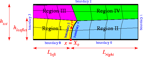
Sketch illustrating the algebraic node update procedure.

The implementation of the node update functions is straightforward and can be found in the source files

src/meshes/channel_with_leaflet_mesh.template.h

and

src/meshes/channel_with_leaflet_mesh.template.cc

which also illustrate how the mesh is constructed by inheritance from the SimpleRectangularQuadMesh (the main task being the creation of additional nodes in the interior to "cut open" the mesh along the position of the leaflet). The source files also contain other versions of the mesh in which the node update is performed with Domain/MacroElements, using the technique described in another tutorial.

Exercise

With the node update strategy illustrated above, the position of all nodes in the fluid mesh has to be updated when the leaflet moves. This is not a particular problem in the current application where the node-update is only performed once per timestep. However, in the corresponding FSI problem , the approach is costly because of the of large number of shape derivatives to be computed.

As an exercise, we suggest to make the node-update procedure more efficient by sub-dividing the regions upstream and downstream of the leaflet into a central section in which the nodes move in response to the motion of the leaflet (the old regions I-IV) and two additional regions (regions V and VI) in which they remain stationary. This is easy because, as explained elsewhere, all AlgebraicNodes already have a default node update function that leaves them stationary.

A better node update strategy.

Acknowledgements

This code was originally developed by Floraine Cordier.

Source files for this tutorial

The source files for this tutorial are located in the directory:

demo_drivers/navier_stokes/channel_with_leaflet/
The driver code is:

demo_drivers/navier_stokes/channel_with_leaflet/channel_with_leaflet.cc

PDF file

A pdf version of this document is available.