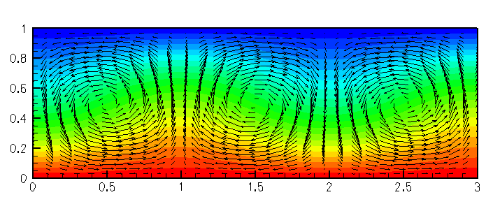
Steady Convection Rolls: contours of temperature and the vector velocity field for a two-dimensional domain heated from below at Ra = 1800

We study convection of an incompressible Newtonian fluid heated from below in a two-dimensional domain of height : the Bénard problem. The lower wall is maintained at a temperature $\theta_{bottom}$ and the upper wall is maintained at a temperature $\theta_{top}$ , where $\theta_{bottom} > \theta_{top}$ . The governing equations are the (2D) Navier–Stokes equations under the Boussinesq approximation, in which all variations in physical properties with temperature are neglected, apart from that of the density in the gravitational-body-force term in the momentum equations. This "buoyancy" term is given by

$\Delta\rho G^{*}_{i},$

where $\Delta\rho$ is the variation in density and $G^{*}_{i}$ is the -th component of the gravitational body force. Under the additional assumption that variations in temperature are small, we can use the linear relationship

$\Delta\rho = -\alpha\rho_{0}(\theta^{*} - \theta_{0}),$

where $\alpha$ is the coefficient of thermal expansion of the fluid, $\theta^{*}$ is the (dimensional) temperature and $\rho_{0}$ is the density at the reference temperature $\theta_{0}$ .

The equations governing the fluid motion are thus the Navier–Stokes equations with the inclusion of the additional buoyancy term. In Cartesian coordinates, we have

$\rho_{0} \left (\frac{\partial u^{*}_i}{\partial t^{*}} + u^{*}_j \frac{\partial u^{*}_i}{\partial x^{*}_j} \right) = - \frac{\partial p^{*}}{\partial x^{*}_i} + \left[\rho_{0} - \alpha\rho_{0}(\theta^{*} - \theta_{0})\right] G^{*}_i + \mu_{0} \frac{\partial }{\partial x^{*}_j} \left[ \frac{\partial u^{*}_i}{\partial x^{*}_j} + \frac{\partial u^{*}_j}{\partial x^{*}_i} \right],$

and

$\frac{\partial u^{*}_i}{\partial x^{*}_i} = 0.$

Here, $u^{*}_{i}$ is the -th (dimensional) velocity component and $x^{*}_{i}$ is the position in the -th coordinate direction; $\mu_{0}$ is the dynamic viscosity of the fluid at the reference temperature and $t^{*}$ is the dimensional time.

The equation that governs the evolution of the temperature field is the advection-diffusion equation where the "wind" is the fluid velocity. Thus,

$\frac{\partial \theta^{*}}{\partial t^{*}} + u^{*}_{j}\frac{\partial \theta^{*}}{\partial x^{*}_{j}} = \kappa\frac{\partial}{\partial x^{*}_{j}}\left(\frac{\partial \theta^{*}}{\partial x^{*}_{j}}\right),$

where $\kappa$ is the (constant) thermal diffusivity of the fluid.

We choose the height of the domain, , as the length scale and let the characteristic thermal diffusion speed over that length, $\kappa/H$ , be the velocity scale, so that the Péclet number, $Pe = UH/\kappa = 1$ . The fluid pressure is non-dimensionalised on the viscous scale, $\mu_{0} \kappa/H^{2}$ , and the hydrostatic pressure gradient is included explicitly, so that we work with the dimensionless excess pressure. The temperature is non-dimensionalised so that it is -0.5 at the upper (cooled) wall and 0.5 at the bottom (heated) wall and the reference temperature is then $\theta_{0} = (\theta_{top} + \theta_{bottom})/2$ . Finally, the timescale is chosen to be the thermal diffusion timescale, $\kappa/H^{2}$ . Hence

$x^{*}_{i} = x_{i} H, \quad u^{*}_{i} = u_{i} \kappa/H, \quad p^{*} = -\rho_{0} g H x_{2} + \frac{\mu_{0}\kappa}{H^{2}}p,\quad \theta^{*} = \theta_{0} + \theta(\theta_{bottom} - \theta_{top}), \quad t^{*} = \frac{\kappa}{H^{2}}t.$

The governing equations become

$Pr^{-1}\left(\frac{\partial u_i}{\partial t} + u_j \frac{\partial u_i}{\partial x_j} \right) = - \frac{\partial p}{\partial x_i} - Ra \theta G_i + \frac{\partial }{\partial x_j} \left[ \frac{\partial u_i}{\partial x_j} + \frac{\partial u_j}{\partial x_i} \right],$

$\frac{\partial u_i}{\partial x_i} = 0,$

and

$\frac{\partial \theta}{\partial t} + u_{j}\frac{\partial \theta}{\partial x_{j}} = \frac{\partial}{\partial x_{j}}\left(\frac{\partial \theta}{\partial x_{j}}\right),$

The appropriate dimensionless numbers are the Prandtl number $Pr = \frac{\nu}{\kappa}$ , and the Rayleigh number, $Ra = \frac{\alpha (\theta_{bottom} - \theta_{top})g H^{3}}{\nu\kappa}$ ; is the acceleration due to gravity and $\nu = \mu_{0}/\rho_{0}$ is the kinematic viscosity of the fluid.

We consider the solution of this coupled set of equations in a two-dimensional domain $0 \leq x_{1} \leq 3$ , $0 \leq x_{2} \leq 1$ . The boundary conditions are no-slip at the top and bottom walls

$u_{1} = u_{2} = 0 \quad\mbox{on } x_{2} = 0, 1;$

constant temperature at the top and bottom walls (heated from below)

$\theta = 0.5 \quad\mbox{on } x_{2}=0 \quad\mbox{and}\quad \theta = -0.5 \quad\mbox{on } x_{2} = 1;$

and symmetry boundary conditions at the sides:

$u_{1} = 0,\quad \frac{\partial u_{2}}{\partial x_{1}} = 0, \quad \mbox{ and } \frac{\partial \theta}{\partial x_{1}} = 0 \quad\mbox{on } x_{1} = 0,3.$

We assume that gravity acts vertically downward so that $G_{1} = 0$ and $G_{2} = -1$ .

There is a trivial steady-state solution that consists of a linearly-varying temperature field balanced by a quadratic pressure field:

$u_{1} = u_{2} = 0, \quad \theta = 0.5 - x_2, \quad p = P_{0} + 0.5 \ Ra \ x_{2} \left(1 - x_{2}\right).$

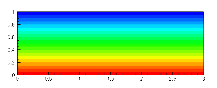
The base flow: no flow and a linear temperature distribution

A linear stability analysis shows that this solution becomes unstable via an up-down, symmetry-breaking, pitchfork bifurcation at a critical Rayleigh number of $Ra_{crit} \approx 1708$ with a critical wavenumber of $k \approx 3.11,$ see for example Hydrodynamic and Hydromagnetic Stability by S. Chandrasekhar OUP (1961). Thus, for there are three possible steady solutions, the (unstable) trivial steady state and two (stable) symmetry-broken states. In principle, all three states can be computed directly by solving the steady equations. However, we typically find that if the steady computation is started with a zero initial guess for the velocity and temperature, the Newton method converges to the trivial state. In order to demonstrate that this state is indeed unstable we therefore apply a time-dependent, mass-conserving perturbation to the vertical velocity at the upper wall and time-march the system while rapidly reducing the size of the perturbation. The system then evolves towards the nontrivial steady state as shown in the animation from which the plots shown above were extracted. (In the next tutorial where we discuss the adaptive solution of this problem we shall demonstrate an alternative technique for obtaining this solutions).

Note that by choosing our domain of a particular size and applying symmetry conditions at the sidewalls we are only able to realise a discrete set of wavelengths (those that exactly fit into the box). At the chosen Rayleigh number, 1800, only one of these modes is unstable; that of wavelength 2.

Global parameters and functions

The problem contains three global parameters, the Péclet number, the Prandtl number and the Rayleigh number which we define in a namespace, as usual. In fact, is the natural dimensionless grouping, and so we use the inverse Prandtl number as our variable.

//======start_of_namespace============================================
/// Namespace for the physical parameters in the problem
//====================================================================
namespace Global_Physical_Variables
{
 /// Peclet number (identically one from our non-dimensionalisation)
 double Peclet=1.0;
 
 /// 1/Prandtl number
 double Inverse_Prandtl=1.0;
 
 /// Rayleigh number, set to be greater than 
 /// the threshold for linear instability
 double Rayleigh = 1800.0;
 
 /// Gravity vector
 Vector<double> Direction_of_gravity(2);
  
} // end_of_namespace

The driver code

In the driver code we set the direction of gravity and construct our problem, using the new BuoyantQCrouzeixRaviartElement, a multi-physics element, created by combining the QCrouzeixRaviart Navier-Stokes elements with the QAdvectionDiffusion elements via multiple inheritance. (Details of the element's implementation are discussed in the section Creating the new BuoyantQCrouzeixRaviartElement class below.)

//=======start_of_main================================================
/// Driver code for 2D Boussinesq convection problem
//====================================================================
int main(int argc, char **argv)
{
 
 // Set the direction of gravity
 Global_Physical_Variables::Direction_of_gravity[0] = 0.0;
 Global_Physical_Variables::Direction_of_gravity[1] = -1.0;
 
 //Construct our problem
 ConvectionProblem<BuoyantQCrouzeixRaviartElement<2> > problem;

We assign the boundary conditions at the time and initially perform a single steady solve to obtain the trivial (and temporally unstable) trivial solution; see the section Comments for a more detailed discussion of the Problem::steady_newton_solve() function.

 // Apply the boundary condition at time zero
 problem.set_boundary_conditions(0.0);
 
 //Perform a single steady Newton solve
 problem.steady_newton_solve();
 
 //Document the solution
 problem.doc_solution();

The result of this calculation is the trivial symmetric base flow. We next timestep the system using the (unstable) steady solution as the initial condition. As time increases, the flow evolves to one of the stable asymmetric solutions, as shown in the animation of the results. As usual, we only perform a few timesteps when the code is used as a self-test, i.e. if any command-line parameters are passed to the driver code.

 //Set the timestep
 double dt = 0.1;
 
 //Initialise the value of the timestep and set an impulsive start
 problem.assign_initial_values_impulsive(dt);
 
 //Set the number of timesteps to our default value
 unsigned n_steps = 200;
 
 //If we have a command line argument, perform fewer steps 
 //(used for self-test runs)
 if(argc > 1) {n_steps = 5;}
 
 //Perform n_steps timesteps
 for(unsigned i=0;i<n_steps;++i)
  {
   problem.unsteady_newton_solve(dt);
   problem.doc_solution();
  }
 
} // end of main

The problem class

The problem class contains five non-trivial functions: the constructor, the fix_pressure(...) function, as well as the functions set_boundary_conditions(...), actions_before_implicit_timestep(...) and doc_solution(...), all discussed below.

The constructor

We pass the element type as a template parameter to the problem constructor, which has no arguments. The constructor creates a BFD<2> timestepper and builds a RectangularQuadMesh of $8\times 8$ elements.

//===========start_of_constructor=========================================
/// Constructor for convection problem
//========================================================================
template<class ELEMENT>
ConvectionProblem<ELEMENT>::ConvectionProblem()
{
 //Allocate a timestepper
 add_time_stepper_pt(new BDF<2>);
 
 // Set output directory
 Doc_info.set_directory("RESLT");
 
 // # of elements in x-direction
 unsigned n_x=8;
 
 // # of elements in y-direction
 unsigned n_y=8;
 
 // Domain length in x-direction
 double l_x=3.0;
 
 // Domain length in y-direction
 double l_y=1.0;
 
 // Build a standard rectangular quadmesh
 Problem::mesh_pt() = 
  new RectangularQuadMesh<ELEMENT>(n_x,n_y,l_x,l_y,time_stepper_pt());

Next, the boundary constraints are imposed. We pin all velocities and the temperature on the top and bottom walls and pin only the horizontal velocity on the sidewalls. Since the domain is enclosed, the pressure is only determined up the an arbitrary constant. We resolve this ambiguity by pinning a single pressure value, using the fix_pressure(...) function.

 // Set the boundary conditions for this problem: All nodes are
 // free by default -- only need to pin the ones that have Dirichlet 
 // conditions here
 
 //Loop over the boundaries
 unsigned num_bound = mesh_pt()->nboundary();
 for(unsigned ibound=0;ibound<num_bound;ibound++)
  {
   //Set the maximum index to be pinned (all values by default)
   unsigned val_max=3;
   //If we are on the side-walls, the v-velocity and temperature
   //satisfy natural boundary conditions, so we only pin the
   //first value
   if((ibound==1) || (ibound==3)) {val_max=1;}
 
   //Loop over the number of nodes on the boundry
   unsigned num_nod= mesh_pt()->nboundary_node(ibound);
   for (unsigned inod=0;inod<num_nod;inod++)
    {
     //Loop over the desired values stored at the nodes and pin
     for(unsigned j=0;j<val_max;j++)
      {
       mesh_pt()->boundary_node_pt(ibound,inod)->pin(j);
      }
    }
  }
 
 //Pin the zero-th pressure dof in element 0 and set its value to
 //zero:
 fix_pressure(0,0,0.0);

We complete the build of the elements by setting the pointers to the physical parameters and finally assign the equation numbers

 unsigned n_element = mesh_pt()->nelement();
 for(unsigned i=0;i<n_element;i++)
  {
   // Upcast from GeneralsedElement to the present element
   ELEMENT *el_pt = dynamic_cast<ELEMENT*>(mesh_pt()->element_pt(i));
 
   // Set the Peclet number
   el_pt->pe_pt() = &Global_Physical_Variables::Peclet;
 
   // Set the Peclet number multiplied by the Strouhal number
   el_pt->pe_st_pt() =&Global_Physical_Variables::Peclet;
 
   // Set the Reynolds number (1/Pr in our non-dimensionalisation)
   el_pt->re_pt() = &Global_Physical_Variables::Inverse_Prandtl;
 
   // Set ReSt (also 1/Pr in our non-dimensionalisation)
   el_pt->re_st_pt() = &Global_Physical_Variables::Inverse_Prandtl;
 
   // Set the Rayleigh number
   el_pt->ra_pt() = &Global_Physical_Variables::Rayleigh;
 
   //Set Gravity vector
   el_pt->g_pt() = &Global_Physical_Variables::Direction_of_gravity;
 
   //The mesh is fixed, so we can disable ALE
   el_pt->disable_ALE();
  }
 
 // Setup equation numbering scheme
 cout <<"Number of equations: " << assign_eqn_numbers() << endl; 
 
} // end of constructor

The function set_boundary_conditions(...)

In order to examine the stability of the symmetric state, we impose a time-dependent boundary condition that transiently perturbs the vertical velocity field at the upper boundary. Our boundary condition is

$u_{2}\big|_{x_2=1} = \epsilon \ t \ \mbox{e}^{-t} \sin(2\pi x_{1}/3),$

where $\epsilon \ll 1$ . The perturbation is zero at , tends to zero as $t\to\infty$ , and is mass conserving. This is implemented in the function below

//===========start_of_set_boundary_conditions================
/// Set the boundary conditions as a function of continuous 
/// time
//===========================================================
template<class ELEMENT>
void ConvectionProblem<ELEMENT>::set_boundary_conditions(
 const double &time)
{
 // Loop over the boundaries
 unsigned num_bound = mesh_pt()->nboundary();
 for(unsigned ibound=0;ibound<num_bound;ibound++)
  {
   // Loop over the nodes on boundary 
   unsigned num_nod=mesh_pt()->nboundary_node(ibound);
   for(unsigned inod=0;inod<num_nod;inod++)
    {
     // Get pointer to node
     Node* nod_pt=mesh_pt()->boundary_node_pt(ibound,inod);
 
     //Set the number of velocity components
     unsigned vel_max=2;
 
     //If we are on the side walls we only set the x-velocity.
     if((ibound==1) || (ibound==3)) {vel_max = 1;}
 
     //Set the pinned velocities to zero
     for(unsigned j=0;j<vel_max;j++) {nod_pt->set_value(j,0.0);}
 
     //If we are on the top boundary
     if(ibound==2) 
      {
       //Set the temperature to -0.5 (cooled)
       nod_pt->set_value(2,-0.5);
 
       //Add small velocity imperfection if desired
       double epsilon = 0.01;
 
       //Read out the x position
       double x = nod_pt->x(0);
 
       //Set a sinusoidal perturbation in the vertical velocity
       //This perturbation is mass conserving
       double value = sin(2.0*MathematicalConstants::Pi*x/3.0)*
        epsilon*time*exp(-time);
       nod_pt->set_value(1,value);
      }
 
     //If we are on the bottom boundary, set the temperature
     //to 0.5 (heated)
     if(ibound==0) {nod_pt->set_value(2,0.5);}
    }
  }
} // end_of_set_boundary_conditions

The function fix_pressure(...)

This function is a simple wrapper to the element's fix_pressure(...) function.

 /// Fix pressure in element e at pressure dof pdof and set to pvalue
 void fix_pressure(const unsigned &e, const unsigned &pdof, 
                   const double &pvalue)
  {
   //Cast to specific element and fix pressure
   dynamic_cast<ELEMENT*>(mesh_pt()->element_pt(e))->
    fix_pressure(pdof,pvalue);
  } // end_of_fix_pressure

The function actions_before_implicit_timestep()

This function is used to ensure that the time-dependent boundary conditions are set to the correct value before solving the problem at the next time level.

 /// Actions before the timestep (update the the time-dependent 
 /// boundary conditions)
 void actions_before_implicit_timestep() 
  {
   set_boundary_conditions(time_pt()->time());
  }

The function doc_solution(...)

This function writes the complete velocity, pressure and temperature fields to a file in the output directory.

//===============start_doc_solution=======================================
/// Doc the solution
//========================================================================
template<class ELEMENT>
void ConvectionProblem<ELEMENT>::doc_solution()
{ 
 //Declare an output stream and filename
 ofstream some_file;
 char filename[100];
 
 // Number of plot points: npts x npts
 unsigned npts=5;
 
 // Output solution 
 //-----------------
 sprintf(filename,"%s/soln%i.dat",Doc_info.directory().c_str(),
         Doc_info.number());
 some_file.open(filename);
 mesh_pt()->output(some_file,npts);
 some_file.close();
 
 Doc_info.number()++;
} // end of doc

Creating the new BuoyantQCrouzeixRaviartElement class

The sketch below illustrates how the new multi-physics BuoyantQCrouzeixRaviartElement is constructed by multiple inheritance from the two existing single-physics elements:

Sketch illustrating the construction of the BuoyantQCrouzeixRaviartElement by multiple inheritance.

The nine-noded two-dimensional QCrouzeixRaviartElement is based on a nine-node quadrilateral geometric FiniteElement from the QElement family. All of its Nodes store two values, the horizontal and vertical velocity, respectively. The element also stores internal Data which represents the (discontinuous) pressure degrees of freedom; in the sketch this Data is represented by the dashed box.
The two-dimensional QAdvectionDiffusionElement is based on the same geometric FiniteElement and stores one value (the temperature, $\theta$ ) at each Node.

Both elements are fully-functional and provide their contributions to the global system of nonlinear algebraic equations that is solved by Newton's method via the two member functions fill_in_contribution_to_residuals(...) and
fill_in_contribution_to_jacobian(...).

The QAdvectionDiffusionElement's member function fill_in_contribution_to_residuals(...) computes the element's contribution to the global residual vector for a given "wind". The "wind" is specified by its virtual member function get_wind_adv_diff(...) and in the single-physics advection diffusion problems studied so far, the "wind" tended to specified a priori by the user. The element's
member function fill_in_contribution_to_jacobian(...) computes the elemental Jacobian matrix, i.e. the derivatives of the elemental residual vector with respect to its unknown nodal values (the temperatures).
Similarly, the QCrouzeixRaviartElement's member function fill_in_contribution_to_residuals(...) computes the element's contribution to the global residual vector for a given body force. The body force is specified by its virtual member function get_body_force_nst(...) and in the single-physics Navier-Stokes problems studied so far, the body force tended to specified a priori by the user. The element's member function fill_in_contribution_to_jacobian(...) computes the elemental Jacobian matrix, i.e. the derivatives of the elemental residual vector with respect to its unknown nodal and internal values (the velocities and the pressure).

When combining the two single-physics elements to a multi-physics element, we have to take the interaction between the constituent equations into account: In the coupled problem the "wind" in the advection-diffusion equations is given by the Navier-Stokes velocities, while the body force in the Navier-Stokes equations is a function of the temperature. When implementing these interactions we wish to recycle as much of the elements' existing functionality as possible. This may be achieved by the following straightforward steps:

Construct the combined multi-physics element by multiple inheritance.
Overload the FiniteElement::required_nvalue(...) function to ensure that each Node provides a sufficient amount of storage for the (larger) number of nodal values required in the multi-physics problem.
Overload the constituent element's member functions that indicate which nodal value corresponds to which type of degree of freedom. For instance, in the single-physics advection-diffusion problem, the temperature is stored at the zero-th nodal value whereas in the combined multi-physics element, the temperature is stored as the second value, as shown in the above sketch.
Provide a final overload for the element's fill_in_contribution_to_residuals(...) and fill_in_contribution_to_jacobian(...) functions.
The former simply concatenates the residual vectors computed by the constituent single-physics elements. The latter function is easiest to implement by finite differencing the combined element's residual vector. [A more efficient approach (in terms of cpu time, not necessarily terms of development time!) is to recycle the diagonal blocks computed by the constituent elements's fill_in_contribution_to_jacobian(...) functions and to use finite-differencing only for the off-diagonal (interaction) blocks; see the section Comments a more detailed discussion of this technique.]

That's all! Here is the implementation:

  //======================class definition==============================
  /// A class that solves the Boussinesq approximation of the Navier--Stokes
  /// and energy equations by coupling two pre-existing classes.
  /// The QAdvectionDiffusionElement with bi-quadratic interpolation for the
  /// scalar variable (temperature) and
  /// QCrouzeixRaviartElement which solves the Navier--Stokes equations
  /// using bi-quadratic interpolation for the velocities and a discontinuous
  /// bi-linear interpolation for the pressure. Note that we are free to
  /// choose the order in which we store the variables at the nodes. In this
  /// case we choose to store the variables in the order fluid velocities
  /// followed by temperature. We must, therefore, overload the function
  /// AdvectionDiffusionEquations<DIM>::u_index_adv_diff() to indicate that
  /// the temperature is stored at the DIM-th position not the 0-th. We do not
  /// need to overload the corresponding function in the
  /// NavierStokesEquations<DIM> class because the velocities are stored
  /// first.
  //=========================================================================
  template<unsigned DIM>
  class BuoyantQCrouzeixRaviartElement
    : public virtual QAdvectionDiffusionElement<DIM, 3>,
      public virtual QCrouzeixRaviartElement<DIM>

The class contains a single new physical parameter, the Rayleigh number, as usual referenced by a pointer to a double precision datum,

/// Pointer to a private data member, the Rayleigh number

double* Ra_pt;

with suitable access functions.

    /// Access function for the Rayleigh number (const version)
    const double& ra() const
    {
      return *Ra_pt;
    }
 
    /// Access function for the pointer to the Rayleigh number
    double*& ra_pt()

The constructor calls the constructors of the component classes (QCrouzeixRaviartElement and QAdvectionDiffusionElement) and initialises the value of the Rayleigh number to zero, via a static default parameter value.

    /// Constructor: call the underlying constructors and
    /// initialise the pointer to the Rayleigh number to point
    /// to the default value of 0.0.
    BuoyantQCrouzeixRaviartElement()
      : QAdvectionDiffusionElement<DIM, 3>(), QCrouzeixRaviartElement<DIM>()
    {
      Ra_pt = &Default_Physical_Constant_Value;
    }

We must overload the function FiniteElement::required_nvalue() because the new element will store DIM+1 unknowns at each node: DIM fluid velocity components and the value of the temperature, as shown in the sketch above.

    /// The required number of values stored at the nodes is the sum of
    /// the required values of the two single-physics  elements. Note that this
    /// step is generic for any multi-physics element of this type.
    unsigned required_nvalue(const unsigned& n) const
    {
      return (QAdvectionDiffusionElement<DIM, 3>::required_nvalue(n) +
              QCrouzeixRaviartElement<DIM>::required_nvalue(n));

In the standard single-physics advection-diffusion elements the temperature is the only value stored at the nodes and is stored as value(0). Similarly, in the single-physics Navier–Stokes elements, the fluid velocities are stored in the first DIM nodal values. In our new multi-physics element, we must decide where to store the different variables and then inform the single-physics elements of our choice. As indicated in the above sketch, we choose to store the temperature after the fluid velocities, so that it is value(DIM). The recommended mechanism for communicating the location of the variables to the single-physics elements is to use an index function. Hence, single-physics elements that are to be the components of multi-physics elements must have an index function for their variables. For instance, the function u_index_adv_diff(...) is used in the AdvectionDiffusionEquations class to read out the position (index) at which the advected variable (the temperature) is stored. That function is now overloaded in our multi-physics element:

    /// Overload the index at which the temperature
    /// variable is stored. We choose to store it after the fluid velocities.
    inline unsigned u_index_adv_diff() const
    {
      return DIM;
    }

We need not overload the index function for the fluid velocities because they remain stored in the first DIM positions at the node.

The coupling between the two sets of single-physics equations is achieved by overloading the two functions get_wind_adv_diff(), used in the advection-diffusion equations and get_body_force_nst(), used in the Navier–Stokes equations

    /// Overload the wind function in the advection-diffusion equations.
    /// This provides the coupling from the Navier--Stokes equations to the
    /// advection-diffusion equations because the wind is the fluid velocity.
    void get_wind_adv_diff(const unsigned& ipt,
                           const Vector<double>& s,
                           const Vector<double>& x,
                           Vector<double>& wind) const
    {
      // The wind function is simply the velocity at the points
      this->interpolated_u_nst(s, wind);
    }

    /// Overload the body force in the Navier-Stokes equations
    /// This provides the coupling from the advection-diffusion equations
    /// to the Navier--Stokes equations, the body force is the
    /// temperature multiplied by the Rayleigh number acting in the
    /// direction opposite to gravity.
    void get_body_force_nst(const double& time,
                            const unsigned& ipt,
                            const Vector<double>& s,
                            const Vector<double>& x,
                            Vector<double>& result)
    {
      // Get the temperature
      const double interpolated_t = this->interpolated_u_adv_diff(s);
 
      // Get vector that indicates the direction of gravity from
      // the Navier-Stokes equations
      Vector<double> gravity(NavierStokesEquations<DIM>::g());
 
      // Temperature-dependent body force:
      for (unsigned i = 0; i < DIM; i++)
      {
        result[i] = -gravity[i] * interpolated_t * ra();
      }

The elemental residual vector is composed of the residuals from the two single-physics elements and we simply call the underlying functions for each element in turn.

    /// Calculate the element's contribution to the residual vector.
    /// Recall that fill_in_* functions MUST NOT initialise the entries
    /// in the vector to zero. This allows us to call the
    /// fill_in_* functions of the constituent single-physics elements
    /// sequentially, without wiping out any previously computed entries.
    void fill_in_contribution_to_residuals(Vector<double>& residuals)
    {
      // Fill in the residuals of the Navier-Stokes equations
      NavierStokesEquations<DIM>::fill_in_contribution_to_residuals(residuals);
 
      // Fill in the residuals of the advection-diffusion eqautions
      AdvectionDiffusionEquations<DIM>::fill_in_contribution_to_residuals(
        residuals);
    }

Finally, we compute the Jacobian matrix by finite-differencing the element's combined residual vector, using the default implementation of the fill_in_contribution_to_jacobian(...) function in the FiniteElement base class:

    /// Compute the element's residual vector and the Jacobian matrix.
    /// Jacobian is computed by finite-differencing.
    void fill_in_contribution_to_jacobian(Vector<double>& residuals,
                                          DenseMatrix<double>& jacobian)
    {
      // This function computes the Jacobian by finite-differencing
      FiniteElement::fill_in_contribution_to_jacobian(residuals, jacobian);
    }

Finally, we overload the output function to print the fluid velocities, the fluid pressure and the temperature.

    // Start of output function
    void output(std::ostream& outfile, const unsigned& nplot)
    {
      // vector of local coordinates
      Vector<double> s(DIM);
 
      // Tecplot header info
      outfile << this->tecplot_zone_string(nplot);
 
      // Loop over plot points
      unsigned num_plot_points = this->nplot_points(nplot);
      for (unsigned iplot = 0; iplot < num_plot_points; iplot++)
      {
        // Get local coordinates of plot point
        this->get_s_plot(iplot, nplot, s);
 
        // Output the position of the plot point
        for (unsigned i = 0; i < DIM; i++)
        {
          outfile << this->interpolated_x(s, i) << " ";
        }
 
        // Output the fluid velocities at the plot point
        for (unsigned i = 0; i < DIM; i++)
        {
          outfile << this->interpolated_u_nst(s, i) << " ";
        }
 
        // Output the fluid pressure at the plot point
        outfile << this->interpolated_p_nst(s) << " ";
 
        // Output the temperature (the advected variable) at the plot point
        outfile << this->interpolated_u_adv_diff(s) << std::endl;
      }
      outfile << std::endl;
 
      // Write tecplot footer (e.g. FE connectivity lists)
      this->write_tecplot_zone_footer(outfile, nplot);
    } // End of output function

Comments and Exercises

Comments

The steady_newton_solve()function:

In most previous examples we have encountered two main interfaces to oomph-lib's Newton solver:
- The function Problem::newton_solve() employs Newton's method to solve the system of nonlinear algebraic equations arising from the Problem's discretisation. The current Data values are used as the initial guess for the Newton iteration. On return from this function, all unknown Data values will have been assigned their correct values so that the solution of the problem may be plotted by calls to the elements' output functions. We tended to use this function to solve steady problems.
- Given the solution at time $t = t_{\mbox{orig}}$ , the unsteady Newton solver Problem::unsteady_newton_solve(dt,...) increments time by dt, shifts the "history" values and then computes the solution at the advanced time, $t = t_{\mbox{orig}}$ + dt. On return from this function, all unknown Data values (and the corresponding "history" values) will have been assigned their correct values so that the solution at time $t = t_{\mbox{orig}}$ + dt may be plotted by calls to the elements' output functions. We tended to use this function for unsteady problems.
Inspection of the Problem::unsteady_newton_solve(...) function shows that this function is, in fact, a wrapper around Problem::newton_solve(), and that the latter function solves the discretised equations including any terms that arise from an implicit time-discretisation. The only purpose of the wrapper function is to shift the history values before taking the next timestep. This raises the question how to compute steady solutions (i.e. solutions obtained by setting the time-derivatives in the governing equation to zero) of a Problem that was discretised in a form that allows for timestepping, as in the problem studied here. This is the role of the function Problem::steady_newton_solve(): The function performs the following steps:
1. Disable all TimeSteppers in the Problem by calling their TimeStepper::make_steady() member function.
2. Call the Problem::newton_solve() function to compute the solution of the discretised problem with all time-derivatives set to zero.
3. Re-activate all TimeSteppers (unless they were already in "steady" mode when the function was called).
4. Call the function Problem::assign_initial_values_impulsive() to ensure that the "history" values used by the (now re-activated) TimeSteppers are consistent with an impulsive start from the steady solution just computed.
On return from this function, all unknown Data values (and the corresponding "history" values) will have been assigned their correct values so that the solution just computed is a steady solution to the full unsteady equations.
Optimising the implementation of multi-physics interactions:

The combined multi-physics element discussed above was implemented with just a few straightforward lines of code. The ease of implementation comes at a price, however, and more efficient implementations (in terms of CPU time) are possible:
1. Using finite-differencing only for the off-diagonal terms in the Jacobian matrix:
  
  While the use of finite-differencing in the setup of the Jacobian matrix is convenient, it does not exploit the fact that the constituent single-physics elements already provide analytical (and hence cheaper-to-compute) expressions for the two diagonal blocks in the coupled Jacobian matrix (i.e. the derivatives of the fluid residuals with respect to the fluid variables, and the derivatives of the advection diffusion residuals with respect to the temperature degrees of freedom). It is possible to recycle these entries and to use finite-differencing only to compute the off-diagonal interaction blocks (i.e. the derivatives of the Navier-Stokes residuals with respect to the temperature degrees of freedom, and the derivatives of the advection-diffusion residuals with respect to the velocities). In fact, the source code for the BuoyantQCrouzeixRaviartElement includes such an implementation. The full finite-difference-based computation discussed above is used if the code is compiled with the compiler flag USE_FD_JACOBIAN_FOR_BUOYANT_Q_ELEMENT. Finite-differences are used for the off-diagonal blocks only when the compiler flag USE_OFF_DIAGONAL_FD_JACOBIAN_FOR_BUOYANT_Q_ELEMENT is passed. When comparing the two versions of the code, we found the run times for the full finite-difference-based version to be approximately 3-7% higher, depending on the spatial resolution used. The implementation of the more efficient version is still straightforward and can be found in the source code boussinesq_convection.cc.
2. Using an analytic Jacobian matrix:
  
  As discussed above, the re-use of the analytic expressions for the diagonal blocks of the coupled Jacobian matrix is straightforward. For a yet more efficient computation we can assemble analytic expressions for the off-diagonal interaction blocks; although this does require knowledge of precisely how the governing equations were implemented in the single-physics elements. Once again, the source code for the BuoyantQCrouzeixRaviartElement includes such an implementation and, moreover, it is the default behaviour. We found the assembly time for the analytic coupled Jacobian to be approximately 15% of the finite-difference based versions. The implementation is reasonably straightforward and can be found in the source code boussinesq_convection.cc.
3. Complete re-implementation of the coupled element:
  
  Although recycling the analytically computed diagonal blocks in the Jacobian matrix leads to a modest speedup, and the use of analytic off-diagonal blocks to a further speedup, the computation of the coupled residual vector and Jacobian matrix are still somewhat inefficient. This is because the contributions from the Navier-Stokes and advection-diffusion equations are computed in two separate integration loops; and, if computed, the assembly of the analytic off-diagonal terms requires a third integration loop. The only solution to this problem would be to fully merge the source codes for two elements to create a customised element. In the present problem this would not be too difficult, particularly since the derivatives of the Navier-Stokes residuals with respect to the temperature, and the derivatives of the advection-diffusion residuals with respect to the velocities are easy to calculate. However, a reimplementation in this form would break the modularity of the library as any subsequent changes/improvements to the Navier-Stokes elements, say, would have to be added manually to the coupled element. If maximum speed is absolutely essential in your application, you may still wish to choose this option. The existing Navier-Stokes and advection diffusion elements provide the required building blocks for your custom-written coupled element.

Exercises

Confirm that the system is stable, i.e. returns to the trivial state, when .
How does the time-evolution of the system change when no-slip boundary conditions for the fluid velocity are applied on the side boundaries (a rigid box model)?
Re-write the multi-physics elements so that the temperature is stored before the fluid velocities. Confirm that the solution is unchanged in this case.
Assess the computational cost of the finite-difference based setup of the elements' Jacobian matrices by comparing the run times of the two versions of the code.
Try using QTaylorHoodElements as the "fluid" element part of the multi-physics elements. N.B. in this case, the temperature must be stored as the first variable at the nodes because we assume that it is always stored at the same location in every node.

Source files for this tutorial

The source files for this tutorial are located in the directory:

demo_drivers/multi_physics/boussinesq_convection/
The driver code is:

demo_drivers/multi_physics/boussinesq_convection/boussinesq_convection.cc
The source code for the elements is in:

src/multi_physics/boussinesq_elements.h

PDF file

A pdf version of this document is available.