Example problem: Adaptive solution of the 2D advection diffusion equation

In this example we discuss the adaptive solution of the 2D advection-diffusion problem

Two-dimensional advection-diffusion problem in a rectangular domain

Solve

\[ \mbox{Pe}\ \sum_{i=1}^2 w_i \left(x_1,x_2\right) \frac{\partial u}{\partial x_i} = \sum_{i=1}^2 \frac{\partial^2u}{\partial x_i^2} + f(x_1,x_2), \ \ \ \ \ \ \ \ \ \ (1) \]

in the rectangular domain $D =\left\{ (x_1,x_2) \in [0,1] \times [0,2]\right\}$, with Dirichlet boundary conditions

\[ \left. u\right|_{\partial D}=u_0, \ \ \ \ \ \ \ \ \ \ (2) \]

where the Peclet number, $ \mbox{Pe} $ the boundary values, $ u_0$, the source function $ f(x_1,x_2),$
and the components of the "wind" $ w_i(x_1,x_2) \ (i=1,2)$ are given.


We choose the forcing function and the boundary conditions such that

\[ u_0(x_1,x_2) = \tanh(1-\alpha(x_1 \tan\Phi - x_2)), \ \ \ \ \ \ \ \ \ (3) \]

is the exact solution of the problem. For large values of $ \alpha, $ the exact solution approaches a step, oriented at an angle $\Phi$ against the $x_1-$axis.

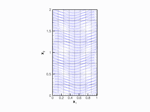
In the computations we will impose the "wind"

\[ \mathbf{w}\left(x_1,x_2 \right) = \left( \begin{array}{c} \sin(6x_2) \\ \cos(6x_1) \end{array} \right), \ \ \ \ \ \ \ \ \ (4) \]

illustrated in this vector plot:

Plot of the wind.

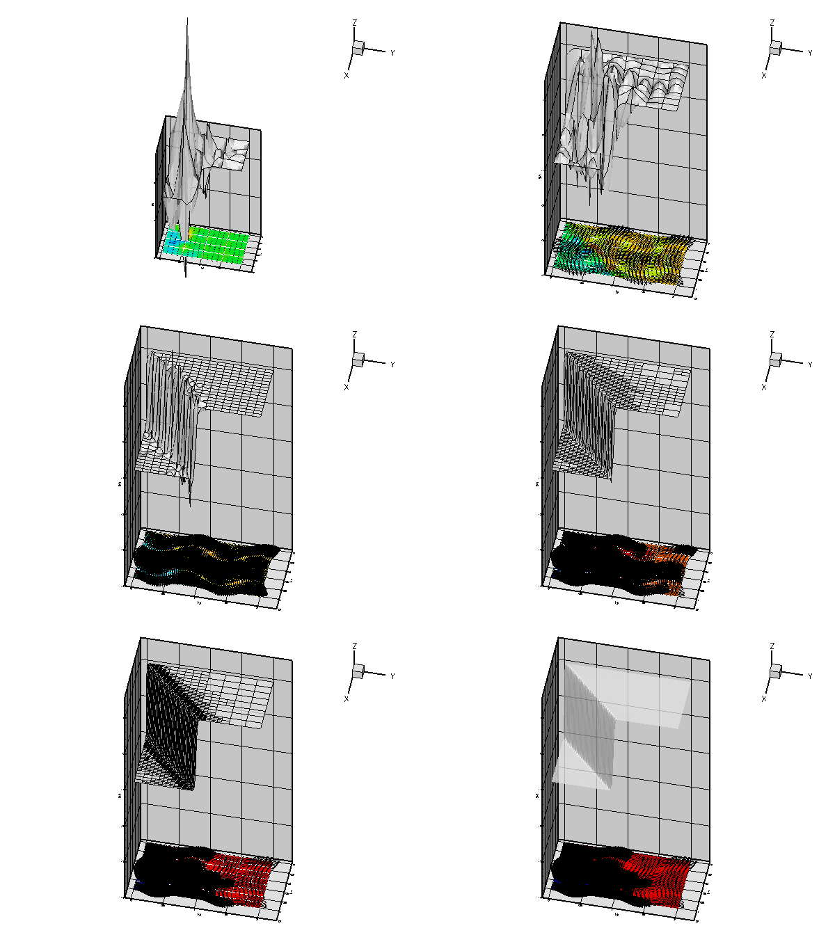
The graph below shows a plot of the solution, computed at various levels of mesh adaptation, for $\Phi=45^\circ, \ \alpha=50 $ and a Peclet number of $ Pe = 200.$

Plot of the forced solution at different levels of mesh refinement.

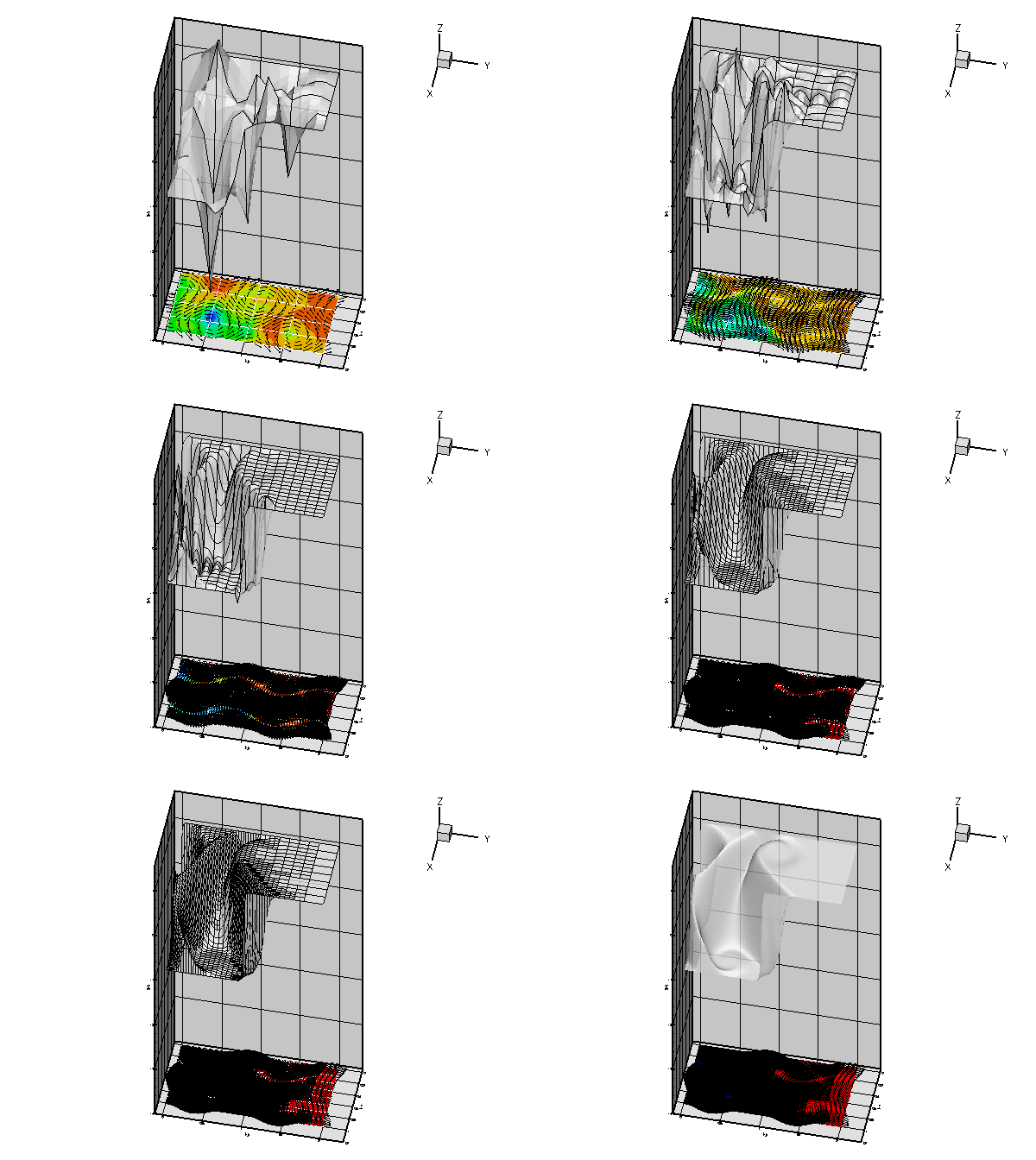
More interesting is the following plot which shows the solution for the same parameter values and boundary conditions, but for a zero forcing function, $ f\equiv 0. $

Plot of the unforced solution at different levels of mesh refinement.

The plot nicely illustrates the physical effects represented by the (unforced) advection diffusion equation. If $ u(x_1,x_2) $ represents the concentration of a chemical that is advected by the velocity field $ {\bf w}$, while being dispersed by molecular diffusion, the advection-diffusion equation describes the steady-state concentration of this chemical. In this context the Peclet number is a measure of the relative importance of advective and diffusive effects. For very small Peclet number, the concentration is determined predominantly by diffusive effects – as $ \mbox{Pe} \to 0$, the advection diffusion equation approaches the Poisson equation. Conversely, at large values of the Peclet number, the concentration is determined predominantly by advective effects. The chemical is "swept along" by the flow and diffusive effects are only important in thin "boundary" or "shear" layers in which the concentration varies over short lengthscales. These can be seen clearly in the most finely resolved solution above.


The driver code

Overall, the structure of the driver code is very similar to that in the corresponding Poisson example. The only difference is that we have to specify function pointers to the source and the "wind" functions, which are passed to the problem constructor. We create the problem, perform a self-test, set the global parameters that affect the solution and solve the problem using oomph-lib's "black-box" adaptive Newton solver.

//===== start_of_main=====================================================
/// Driver code for 2D AdvectionDiffusion problem
//========================================================================
int main()
{
//Set up the problem
//------------------
// Create the problem with 2D nine-node refineable elements from the
// RefineableQuadAdvectionDiffusionElement family. Pass pointer to
// source and wind function.
RefineableAdvectionDiffusionProblem<RefineableQAdvectionDiffusionElement<2,
// Check if we're ready to go:
//----------------------------
cout << "\n\n\nProblem self-test ";
if (problem.self_test()==0)
{
cout << "passed: Problem can be solved." << std::endl;
}
else
{
throw OomphLibError("Self test failed",
OOMPH_CURRENT_FUNCTION,
OOMPH_EXCEPTION_LOCATION);
}
// Set the orientation of the "step" to 45 degrees
// Choose a large value for the steepness of the "step"
// Solve the problem, performing up to 4 adptive refinements
problem.newton_solve(4);
//Output the solution
problem.doc_solution();
} // end of main
/////////////////////////////////////////////////////////////////// /////////////////////////////////...
double TanPhi
Parameter for angle of step.
double Alpha
Parameter for steepness of step.
void source_function(const Vector< double > &x_vect, double &source)
Source function required to make the solution above an exact solution.
void wind_function(const Vector< double > &x, Vector< double > &wind)
Wind.
int main()
Driver code for 2D AdvectionDiffusion problem.


Global parameters and functions

The specification of the source function and the exact solution in the namespace TanhSolnForAdvectionDiffusion is similar to that for the Poisson examples. The only difference is the inclusion of the Peclet number and the "wind" function.

//======start_of_namespace============================================
/// Namespace for exact solution for AdvectionDiffusion equation
/// with "sharp" step
//====================================================================
{
/// Peclet number
double Peclet=200.0;
/// Parameter for steepness of step
double Alpha;
/// Parameter for angle of step
double TanPhi;
/// Exact solution as a Vector
void get_exact_u(const Vector<double>& x, Vector<double>& u)
{
u[0]=tanh(1.0-Alpha*(TanPhi*x[0]-x[1]));
}
/// Exact solution as a scalar
void get_exact_u(const Vector<double>& x, double& u)
{
u=tanh(1.0-Alpha*(TanPhi*x[0]-x[1]));
}
/// Source function required to make the solution above an exact solution
void source_function(const Vector<double>& x_vect, double& source)
{
double x=x_vect[0];
double y=x_vect[1];
source =
2.0*tanh(-0.1E1+Alpha*(TanPhi*x-y))*(1.0-pow(tanh(-0.1E1+Alpha*(
TanPhi*x-y)),2.0))*Alpha*Alpha*TanPhi*TanPhi+2.0*tanh(-0.1E1+Alpha*(TanPhi*x-y)
)*(1.0-pow(tanh(-0.1E1+Alpha*(TanPhi*x-y)),2.0))*Alpha*Alpha-Peclet*(-sin(6.0*y
)*(1.0-pow(tanh(-0.1E1+Alpha*(TanPhi*x-y)),2.0))*Alpha*TanPhi+cos(6.0*x)*(1.0-
pow(tanh(-0.1E1+Alpha*(TanPhi*x-y)),2.0))*Alpha);
}
/// Wind
void wind_function(const Vector<double>& x, Vector<double>& wind)
{
wind[0]=sin(6.0*x[1]);
wind[1]=cos(6.0*x[0]);
}
} // end of namespace
Namespace for exact solution for AdvectionDiffusion equation with "sharp" step.
void get_exact_u(const Vector< double > &x, Vector< double > &u)
Exact solution as a Vector.


The problem class

The problem class is very similar to those used in the corresponding Poisson examples. The only change is that we use the function Problem::actions_before_adapt() to document the progress of the automatic spatial adaptation. For this purpose, we store a DocInfo as private member data in the Problem. This allows us to increment the counter that labels the output files, accessible from DocInfo::number(), whenever a new solution has been documented.

//====== start_of_problem_class=======================================
/// 2D AdvectionDiffusion problem on rectangular domain, discretised
/// with refineable 2D QAdvectionDiffusion elements. The specific type
/// of element is specified via the template parameter.
//====================================================================
template<class ELEMENT>
{
public:
/// Constructor: Pass pointer to source and wind functions
AdvectionDiffusionEquations<2>::AdvectionDiffusionSourceFctPt source_fct_pt,
AdvectionDiffusionEquations<2>::AdvectionDiffusionWindFctPt wind_fct_pt);
/// Destructor. Empty
/// Update the problem specs before solve: Reset boundary conditions
/// to the values from the tanh solution.
/// Update the problem after solve (empty)
/// Actions before adapt: Document the solution
{
// Doc the solution
// Increment label for output files
Doc_info.number()++;
}
/// Doc the solution.
void doc_solution();
/// Overloaded version of the problem's access function to
/// the mesh. Recasts the pointer to the base Mesh object to
/// the actual mesh type.
RefineableRectangularQuadMesh<ELEMENT>* mesh_pt()
{
return dynamic_cast<RefineableRectangularQuadMesh<ELEMENT>*>(
Problem::mesh_pt());
}
private:
/// DocInfo object
DocInfo Doc_info;
/// Pointer to source function
AdvectionDiffusionEquations<2>::AdvectionDiffusionSourceFctPt Source_fct_pt;
/// Pointer to wind function
AdvectionDiffusionEquations<2>::AdvectionDiffusionWindFctPt Wind_fct_pt;
}; // end of problem class
void actions_before_adapt()
Actions before adapt: Document the solution.
RefineableAdvectionDiffusionProblem(AdvectionDiffusionEquations< 2 >::AdvectionDiffusionSourceFctPt source_fct_pt, AdvectionDiffusionEquations< 2 >::AdvectionDiffusionWindFctPt wind_fct_pt)
Constructor: Pass pointer to source and wind functions.
void actions_before_newton_solve()
Update the problem specs before solve: Reset boundary conditions to the values from the tanh solution...
AdvectionDiffusionEquations< 2 >::AdvectionDiffusionSourceFctPt Source_fct_pt
Pointer to source function.
void actions_after_newton_solve()
Update the problem after solve (empty)
AdvectionDiffusionEquations< 2 >::AdvectionDiffusionWindFctPt Wind_fct_pt
Pointer to wind function.
RefineableRectangularQuadMesh< ELEMENT > * mesh_pt()
Overloaded version of the problem's access function to the mesh. Recasts the pointer to the base Mesh...
~RefineableAdvectionDiffusionProblem()
Destructor. Empty.


The Problem constructor

The constructor is practically identical to the constructors used in the various Poisson examples. We specify the output directory in the Problem's DocInfo object, create the mesh and an error estimator, and apply the boundary conditions by pinning the nodal values on the Dirichlet boundaries.

//=====start_of_constructor===============================================
/// Constructor for AdvectionDiffusion problem: Pass pointer to
/// source function.
//========================================================================
template<class ELEMENT>
AdvectionDiffusionEquations<2>::AdvectionDiffusionSourceFctPt source_fct_pt,
AdvectionDiffusionEquations<2>::AdvectionDiffusionWindFctPt wind_fct_pt)
: Source_fct_pt(source_fct_pt), Wind_fct_pt(wind_fct_pt)
{
// Set output directory
Doc_info.set_directory("RESLT");
// Setup mesh
// # of elements in x-direction
unsigned n_x=4;
// # of elements in y-direction
unsigned n_y=4;
// Domain length in x-direction
double l_x=1.0;
// Domain length in y-direction
double l_y=2.0;
// Build and assign mesh
Problem::mesh_pt() =
new RefineableRectangularQuadMesh<ELEMENT>(n_x,n_y,l_x,l_y);
// Create/set error estimator
mesh_pt()->spatial_error_estimator_pt()=new Z2ErrorEstimator;
// Set the boundary conditions for this problem: All nodes are
// free by default -- only need to pin the ones that have Dirichlet
// conditions here
unsigned num_bound = mesh_pt()->nboundary();
for(unsigned ibound=0;ibound<num_bound;ibound++)
{
unsigned num_nod= mesh_pt()->nboundary_node(ibound);
for (unsigned inod=0;inod<num_nod;inod++)
{
mesh_pt()->boundary_node_pt(ibound,inod)->pin(0);
}
} // end loop over boundaries

We complete the problem setup by passing the function pointers to the source and wind functions, and the pointer to the Peclet number to the elements. Finally, we set up the equation numbering scheme.

// Complete the build of all elements so they are fully functional
// Loop over the elements to set up element-specific
// things that cannot be handled by the (argument-free!) ELEMENT
// constructor: Pass pointer to source function
unsigned n_element = mesh_pt()->nelement();
for(unsigned i=0;i<n_element;i++)
{
// Upcast from GeneralsedElement to the present element
ELEMENT *el_pt = dynamic_cast<ELEMENT*>(mesh_pt()->element_pt(i));
//Set the source function pointer
el_pt->source_fct_pt() = Source_fct_pt;
//Set the wind function pointer
el_pt->wind_fct_pt() = Wind_fct_pt;
// Set the Peclet number
}
// Setup equation numbering scheme
cout <<"Number of equations: " << assign_eqn_numbers() << std::endl;
} // end of constructor


Actions before solve

As before, we use the Problem::actions_before_newton_solve() function to set/update the boundary conditions.

//========================================start_of_actions_before_newton_solve===
/// Update the problem specs before solve: (Re-)set boundary conditions
/// to the values from the tanh solution.
//========================================================================
template<class ELEMENT>
{
// How many boundaries are there?
unsigned num_bound = mesh_pt()->nboundary();
//Loop over the boundaries
for(unsigned ibound=0;ibound<num_bound;ibound++)
{
// How many nodes are there on this boundary?
unsigned num_nod=mesh_pt()->nboundary_node(ibound);
// Loop over the nodes on boundary
for (unsigned inod=0;inod<num_nod;inod++)
{
// Get pointer to node
Node* nod_pt=mesh_pt()->boundary_node_pt(ibound,inod);
// Extract nodal coordinates from node:
Vector<double> x(2);
x[0]=nod_pt->x(0);
x[1]=nod_pt->x(1);
// Compute the value of the exact solution at the nodal point
Vector<double> u(1);
// Assign the value to the one (and only) nodal value at this node
nod_pt->set_value(0,u[0]);
}
}
} // end of actions before solve


Post-processing

The function doc_solution(...) is identical to that in the Poisson example. We output the solution, the exact solution and the error.

//===============start_of_doc=============================================
/// Doc the solution
//========================================================================
template<class ELEMENT>
{
ofstream some_file;
char filename[100];
// Number of plot points: npts x npts
unsigned npts=5;
// Output solution
//-----------------
sprintf(filename,"%s/soln%i.dat",Doc_info.directory().c_str(),
Doc_info.number());
some_file.open(filename);
mesh_pt()->output(some_file,npts);
some_file.close();
// Output exact solution
//----------------------
sprintf(filename,"%s/exact_soln%i.dat",Doc_info.directory().c_str(),
Doc_info.number());
some_file.open(filename);
mesh_pt()->output_fct(some_file,npts,TanhSolnForAdvectionDiffusion::get_exact_u);
some_file.close();
// Doc error and return of the square of the L2 error
//---------------------------------------------------
double error,norm;
sprintf(filename,"%s/error%i.dat",Doc_info.directory().c_str(),
Doc_info.number());
some_file.open(filename);
mesh_pt()->compute_error(some_file,TanhSolnForAdvectionDiffusion::get_exact_u,
error,norm);
some_file.close();
// Doc L2 error and norm of solution
cout << "\nNorm of error : " << sqrt(error) << std::endl;
cout << "Norm of solution: " << sqrt(norm) << std::endl << std::endl;
} // end of doc


Comments and Exercises

  1. Explore the change in the character of the solution of the unforced problem when the Peclet number is slowly increased from 0 to 200, say. Note how at small Peclet number, strong diffusive effects smooth out the rapid spatial variations imposed by the boundary conditions. Conversely, at large values of the Peclet number, the behaviour is dominated by advective effects. As a result, in regions where the "wind" is directed into the domain, the value of $ u $ set by the Dirichlet boundary conditions is "swept" into the domain. In regions where the "wind" is directed out of the domain, the value of $ u $ "swept along" by the flow in the interior "clashes" with the value prescribed by the boundary conditions and the solution adjusts itself over a very short length scale, leading to the development of thin "boundary layers".
  2. Explore the character of the solution on coarse meshes at large and small Peclet numbers. Note how at large Peclet numbers the solution on the coarse meshes displays strong "wiggles" throughout the domain. These only disappear once the mesh adaptation fully resolves the regions of rapid variation. We will explore this issue further in another example.


Source files for this tutorial


PDF file

A pdf version of this document is available.