In this example we shall demonstrate

how easy it is to adapt the code for the solution of the driven cavity problem in a square domain, discussed in a previous example , to a different domain shape,
how to apply body forces (e.g. gravity) in a Navier-Stokes problem,
how to switch between the stress-divergence and the simplified forms of the incompressible Navier-Stokes equations.

The example problem

In this example we shall illustrate the solution of the steady 2D Navier-Stokes equations in a modified driven cavity problem: The fluid is contained in a quarter-circle domain and is subject to gravity which acts in the vertical direction. We solve the problem in two different formulations, using the stress-divergence and the simplified form of the Navier-Stokes equations, respectively, and by applying the gravitational body force via the gravity vector, ${\bf G}$ , and via the body force function, ${\bf B}$ , respectively.

Problem 1:The 2D driven cavity problem in a quarter circle domain with gravity,
using the stress-divergence form of the Navier-Stokes equations

Solve

$Re\phantom{i}u_j\frac{\partial u_i}{\partial x_j} = - \frac{\partial p}{\partial x_i} + \frac{Re}{Fr} \, G_i + \frac{\partial }{\partial x_j} \left( \frac{\partial u_i}{\partial x_j} + \frac{\partial u_j}{\partial x_i} \right), \ \ \ \ \ \ \ \ \ \ (1)$

and

$\frac{\partial u_i}{\partial x_i} = 0,$

in the quarter-circle domain $D = \{x_1 \geq 0$ , $x_2 \geq 0$ and $x_1^2+x_2^2 \leq 1 \}$ , subject to the Dirichlet boundary conditions

$\left. \mathbf{u}\right|_{\partial D}=(0,0), \ \ \ \ \ \ \ \ \ \ (2)$

on the curved and left boundaries; and

$\left. \mathbf{u}\right|_{\partial D}=(1,0), \ \ \ \ \ \ \ \ \ \ (3)$

on the bottom boundary, . Gravity acts vertically downwards so that .

When discussing the implementation of the Navier-Stokes equations in an earlier example , we mentioned that oomph-lib allows the incompressible Navier-Stokes equations to be solved in the simplified, rather than the (default) stress-divergence form. We will demonstrate the use of this feature by solving the following problem:

Problem 2:The 2D driven cavity problem in a quarter circle domain with gravity,
using the simplified form of the Navier-Stokes equations

Solve

$Re\phantom{i}u_j\frac{\partial u_i}{\partial x_j} = - \frac{\partial p}{\partial x_i} + B_i + \frac{\partial^2 u_i}{\partial x_j^2}, \ \ \ \ \ \ \ \ \ \ (1)$

and

$\frac{\partial u_i}{\partial x_i} = 0,$

in the quarter-circle domain $D = \{x_1 \geq 0$ , $x_2 \geq 0$ and $x_1^2+x_2^2 \leq 1 \}$ , subject to the Dirichlet boundary conditions

$\left. \mathbf{u}\right|_{\partial D}=(0,0), \ \ \ \ \ \ \ \ \ \ (2)$

on the curved and left boundaries; and

$\left. \mathbf{u}\right|_{\partial D}=(1,0), \ \ \ \ \ \ \ \ \ \ (3)$

on the bottom boundary, . To make this consistent with Problem 1, we define the body force function as .

Note that in Problem 2, the gravitational body force is represented by the body force rather than the gravity vector.

Switching between the stress-divergence and the simplified forms of the Navier-Stokes equations

The two forms of the Navier-Stokes equations differ in the implementation of the viscous terms, which may be represented as

$\frac{\partial^2 u_i}{\partial x_j^2} \mbox{ \ \ \ or \ \ \ } \frac{\partial }{\partial x_j} \left( \frac{\partial u_i}{\partial x_j} + \frac{\partial u_j}{\partial x_i} \right).$

For an incompressible flow, $\partial u_i/\partial x_i = 0$ , both forms are mathematically equivalent but the stress-divergence form is required for problems with free surfaces , or for problems in which traction boundary conditions are to be applied.

In order to be able do deal with both cases, oomph-lib's Navier-Stokes elements actually implement the viscous term as

$\frac{\partial }{\partial x_j} \left( \frac{\partial u_i}{\partial x_j} + \Gamma_i \, \frac{\partial u_j}{\partial x_i} \right).$

By default the components of the vector $\Gamma_i$ , are set to 1.0, so that the stress-divergence form is used. The components $\Gamma_i$ are stored in the static data member

static Vector<double> NavierStokesEquations<DIM>::Gamma

of the NavierStokesEquations<DIM> class which forms the basis for all Navier-Stokes elements in oomph-lib. Its entries are initialised to 1.0. The user may over-write these assignments and thus re-define the values of $\Gamma$ being used for a specific problem. [In principle, it is possible to use stress-divergence form for the first component of the momentum equations, and the simplified form for the second one, say. However, we do not believe that this is a particularly useful/desirable option and have certainly never used such (slightly bizarre) assignments in any of our own computations.]

Solution to problem 1

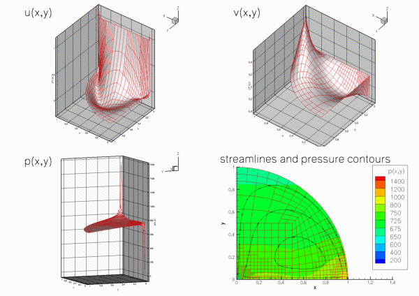
The figure below shows "carpet plots" of the velocity and pressure fields as well as a contour plot of the pressure distribution with superimposed streamlines for Problem 1 at a Reynolds number of and a ratio of Reynolds and Froude numbers (a measure of gravity on the viscous scale) of . The velocity vanishes along the entire domain boundary, apart from the bottom boundary where the moving "lid" imposes a unit tangential velocity which drives a large vortex, centred at $(x_1,x_2) \approx (0.59,0.22)$ . The pressure singularities created by the velocity discontinuities at and are well resolved. The pressure plot shows that away from the singularities, the pressure decreases linearly with , reflecting the effect of the gravitational body forces which acts in the negative direction.

Plot of the velocity and pressure fields for problem 1 with Re=100 and Re/Fr=100, computed with adaptive Taylor-Hood elements.

Solution to problem 2

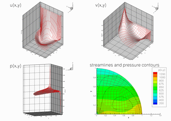
The next figure shows the computational results for Problem 2, obtained from a computation with adaptive Crouzeix-Raviart elements.

Plot of the velocity and pressure fields for problem 2 with Re=100 and Re/Fr=100, computed with adaptive Crouzeix-Raviart elements.

The code

We use a namespace Global_Physical_Variables to define the various parameters: The Reynolds number,

//==start_of_namespace===================================================
/// Namespace for physical parameters
//=======================================================================
namespace Global_Physical_Variables
{
 /// Reynolds number
 double Re=100;

the gravity vector ${\bf G}$ , and the ratio of Reynolds and Froude number, , which represents the ratio of gravitational and viscous forces,

 
 /// Reynolds/Froude number
 double Re_invFr=100;
 
 /// Gravity vector
 Vector<double> Gravity(2);

In Problem 2, gravity is introduced via the body force function ${\bf B}$ which we define such that Problems 1 and 2 are equivalent. (We use the gravity vector ${\bf G} = (0,-1)$ to specify the direction of gravity, while indicating it magnitude by )

 
 /// Functional body force
 void body_force(const double& time, const Vector<double>& x, 
                 Vector<double>& result)
 {
  result[0]=0.0;
  result[1]=-Re_invFr;
 }

Finally we define a body force function, which returns zero values, for use when solving Problem 1.

 
 /// Zero functional body force
 void zero_body_force(const double& time, const Vector<double>& x, 
                      Vector<double>& result)
 {
  result[0]=0.0;
  result[1]=0.0;
 }
 
} // end_of_namespace

The driver code

First we create a DocInfo object to control the output, and set the maximum number of spatial adaptations to three.

//==start_of_main======================================================
/// Driver for QuarterCircleDrivenCavityProblem test problem 
//=====================================================================
int main()
{
 
 // Set output directory and initialise count
 DocInfo doc_info;
 doc_info.set_directory("RESLT");
 
 // Set max. number of black-box adaptation
 unsigned max_adapt=3;

To solve problem 1 we define the direction of gravity, ${\bf G} = (0,-1)$ , and set the entries in the NavierStokesEquations<2>::Gamma vector to , so that the stress-divergence form of the equation is used [In fact, this step is not strictly necessary as it simply re-assigns the default values.]

 
 // Solve problem 1 with Taylor-Hood elements
 //--------------------------------------------
 {
  // Set up downwards-Gravity vector
  Global_Physical_Variables::Gravity[0] = 0.0;
  Global_Physical_Variables::Gravity[1] = -1.0;
  
  // Set up Gamma vector for stress-divergence form
  NavierStokesEquations<2>::Gamma[0]=1;
  NavierStokesEquations<2>::Gamma[1]=1;

Next we build problem 1 using Taylor-Hood elements and passing a function pointer to the zero_body_force(...) function (defined in the namespace Global_Physical_Variables) as the argument.

 
  // Build problem with Gravity vector in stress divergence form, 
  // using zero body force function
  QuarterCircleDrivenCavityProblem<RefineableQTaylorHoodElement<2> > 
   problem(&Global_Physical_Variables::zero_body_force);

Now problem 1 can be solved as in the previous example.

 
  // Solve the problem with automatic adaptation
  problem.newton_solve(max_adapt);
  
  // Step number
  doc_info.number()=0;
 
  // Output solution
  problem.doc_solution(doc_info);  
 
 } // end of problem 1

To solve problem 2 we set the entries in the NavierStokesEquations<2>::Gamma vector to zero (thus choosing the simplified version of the Navier-Stokes equations), define ${\bf G} = (0,0)$ , and pass a function pointer to the body_force(...) function to the problem constructor.

 
 
 
 // Solve problem 2 with Taylor Hood elements
 //--------------------------------------------
 {
  // Set up zero-Gravity vector
  Global_Physical_Variables::Gravity[0] = 0.0;
  Global_Physical_Variables::Gravity[1] = 0.0;
 
  // Set up Gamma vector for simplified form
  NavierStokesEquations<2>::Gamma[0]=0;
  NavierStokesEquations<2>::Gamma[1]=0;
 
  // Build problem with body force function and simplified form,
  // using body force function
  QuarterCircleDrivenCavityProblem<RefineableQTaylorHoodElement<2> >
   problem(&Global_Physical_Variables::body_force);

Problem 2 may then be solved as before.

 
  // Solve the problem with automatic adaptation
  problem.newton_solve(max_adapt);
  
  // Step number
  doc_info.number()=1;
 
  // Output solution
  problem.doc_solution(doc_info);
 
 } // end of problem 2
 
} // end_of_main

The problem class

The problem class is very similar to that used in the previous example , with two exceptions:

We pass a function pointer to the body force function ${\bf B}$ to the constructor and
store the function pointer to the body force function in the problem's private member data.

//==start_of_problem_class============================================
/// Driven cavity problem in quarter circle domain, templated
/// by element type. 
//====================================================================
template<class ELEMENT>
class QuarterCircleDrivenCavityProblem : public Problem
{
 
public:
 
 /// Constructor
 QuarterCircleDrivenCavityProblem(
  NavierStokesEquations<2>::NavierStokesBodyForceFctPt body_force_fct_pt);
 
 /// Destructor: Empty
 ~QuarterCircleDrivenCavityProblem() {}
 
 /// Update the after solve (empty)
 void actions_after_newton_solve() {}
 
 /// Update the problem specs before solve. 
 /// (Re-)set velocity boundary conditions just to be on the safe side...
 void actions_before_newton_solve()
  { 
  // Setup tangential flow along boundary 0:
  unsigned ibound=0; 
  unsigned num_nod= mesh_pt()->nboundary_node(ibound);
  for (unsigned inod=0;inod<num_nod;inod++)
   {
    // Tangential flow
    unsigned i=0;
    mesh_pt()->boundary_node_pt(ibound,inod)->set_value(i,1.0);
    // No penetration
    i=1;
    mesh_pt()->boundary_node_pt(ibound,inod)->set_value(i,0.0);
   }
  
  // Overwrite with no flow along all other boundaries
  unsigned num_bound = mesh_pt()->nboundary();
  for(unsigned ibound=1;ibound<num_bound;ibound++)
   {
    unsigned num_nod= mesh_pt()->nboundary_node(ibound);
    for (unsigned inod=0;inod<num_nod;inod++)
     {
      for (unsigned i=0;i<2;i++)
       {
        mesh_pt()->boundary_node_pt(ibound,inod)->set_value(i,0.0);
       }
     }
   }
  } // end_of_actions_before_newton_solve
 
 
 /// After adaptation: Unpin pressure and pin redudant pressure dofs.
 void actions_after_adapt()
  {
   // Unpin all pressure dofs
   RefineableNavierStokesEquations<2>::
    unpin_all_pressure_dofs(mesh_pt()->element_pt());
 
   // Pin redundant pressure dofs
   RefineableNavierStokesEquations<2>::
    pin_redundant_nodal_pressures(mesh_pt()->element_pt());
   
   // Now pin the first pressure dof in the first element and set it to 0.0
   fix_pressure(0,0,0.0);
  } // end_of_actions_after_adapt
 
 /// Doc the solution
 void doc_solution(DocInfo& doc_info);
 
private:
 
 /// Pointer to body force function
 NavierStokesEquations<2>::NavierStokesBodyForceFctPt Body_force_fct_pt;
 
 /// Fix pressure in element e at pressure dof pdof and set to pvalue
 void fix_pressure(const unsigned &e, const unsigned &pdof, 
                   const double &pvalue)
  {
   //Cast to proper element and fix pressure
   dynamic_cast<ELEMENT*>(mesh_pt()->element_pt(e))->
                          fix_pressure(pdof,pvalue);
  } // end_of_fix_pressure
 
}; // end_of_problem_class

The problem constructor

We store the function pointer to the body force function in the private data member Body_force_fct_pt.

//==start_of_constructor==================================================
/// Constructor for driven cavity problem in quarter circle domain
//========================================================================
template<class ELEMENT>
QuarterCircleDrivenCavityProblem<ELEMENT>::QuarterCircleDrivenCavityProblem(
 NavierStokesEquations<2>::NavierStokesBodyForceFctPt body_force_fct_pt) :
 Body_force_fct_pt(body_force_fct_pt)

As usual the first task is to create the mesh. We now use the RefineableQuarterCircleSectorMesh<ELEMENT>, which requires the creation of a GeomObject to describe geometry of the curved wall: We choose an ellipse with unit half axes (i.e. a unit circle).

{ 
 
 // Build geometric object that parametrises the curved boundary
 // of the domain
 
 // Half axes for ellipse
 double a_ellipse=1.0;
 double b_ellipse=1.0;
 
 // Setup elliptical ring 
 GeomObject* Wall_pt=new Ellipse(a_ellipse,b_ellipse); 
 
 // End points for wall
 double xi_lo=0.0;
 double xi_hi=2.0*atan(1.0);
 
 //Now create the mesh
 double fract_mid=0.5;
 Problem::mesh_pt() = new 
  RefineableQuarterCircleSectorMesh<ELEMENT>(
   Wall_pt,xi_lo,fract_mid,xi_hi);

Next the error estimator is set, the boundary nodes are pinned and the Reynolds number is assigned, as before .

 
 // Set error estimator
 Z2ErrorEstimator* error_estimator_pt=new Z2ErrorEstimator;
 dynamic_cast<RefineableQuarterCircleSectorMesh<ELEMENT>*>(
  mesh_pt())->spatial_error_estimator_pt()=error_estimator_pt;
 
 // Set the boundary conditions for this problem: All nodes are
 // free by default -- just pin the ones that have Dirichlet conditions
 // here: All boundaries are Dirichlet boundaries.
 unsigned num_bound = mesh_pt()->nboundary();
 for(unsigned ibound=0;ibound<num_bound;ibound++)
  {
   unsigned num_nod= mesh_pt()->nboundary_node(ibound);
   for (unsigned inod=0;inod<num_nod;inod++)
    {
     // Loop over values (u and v velocities)
     for (unsigned i=0;i<2;i++)
      {
       mesh_pt()->boundary_node_pt(ibound,inod)->pin(i); 
      }
    }
  } // end loop over boundaries
 
 //Find number of elements in mesh
 unsigned n_element = mesh_pt()->nelement();
 
 // Loop over the elements to set up element-specific 
 // things that cannot be handled by constructor: Pass pointer to Reynolds
 // number
 for(unsigned e=0;e<n_element;e++)
  {
   // Upcast from GeneralisedElement to the present element
   ELEMENT* el_pt = dynamic_cast<ELEMENT*>(mesh_pt()->element_pt(e));
 
   //Set the Reynolds number, etc
   el_pt->re_pt() = &Global_Physical_Variables::Re;

Within this loop we also pass the pointers to , the gravity vector and the body-force function to the elements.

   //Set the Re/Fr
   el_pt->re_invfr_pt() = &Global_Physical_Variables::Re_invFr;
   //Set Gravity vector
   el_pt->g_pt() = &Global_Physical_Variables::Gravity;
   //set body force function
   el_pt->body_force_fct_pt() = Body_force_fct_pt;
 
  } // end loop over elements

The RefineableQuarterCircleSectorMesh<ELEMENT> contains only three elements and therefore provides a very coarse discretisation of the domain. We refine the mesh uniformly twice before pinning the redundant pressure degrees of freedom, pinning a single pressure degree of freedom, and assigning the equation numbers, as before.

 
 // Initial refinement level
 refine_uniformly();
 refine_uniformly();
 
 // Pin redudant pressure dofs
 RefineableNavierStokesEquations<2>::
  pin_redundant_nodal_pressures(mesh_pt()->element_pt());
 
 // Now pin the first pressure dof in the first element and set it to 0.0
 fix_pressure(0,0,0.0);
 
 // Setup equation numbering scheme
 cout <<"Number of equations: " << assign_eqn_numbers() << std::endl; 
 
} // end_of_constructor

Post processing

The post processing function remains the same as in the previous examples .

//==start_of_doc_solution=================================================
/// Doc the solution
//========================================================================
template<class ELEMENT>
void QuarterCircleDrivenCavityProblem<ELEMENT>::doc_solution(DocInfo& doc_info)
{ 
 
 ofstream some_file;
 char filename[100];
 
 // Number of plot points
 unsigned npts=5; 
 
 
 // Output solution 
 sprintf(filename,"%s/soln%i.dat",doc_info.directory().c_str(),
         doc_info.number());
 some_file.open(filename);
 mesh_pt()->output(some_file,npts);
 some_file.close();
 
} // end_of_doc_solution

Comments and Exercises

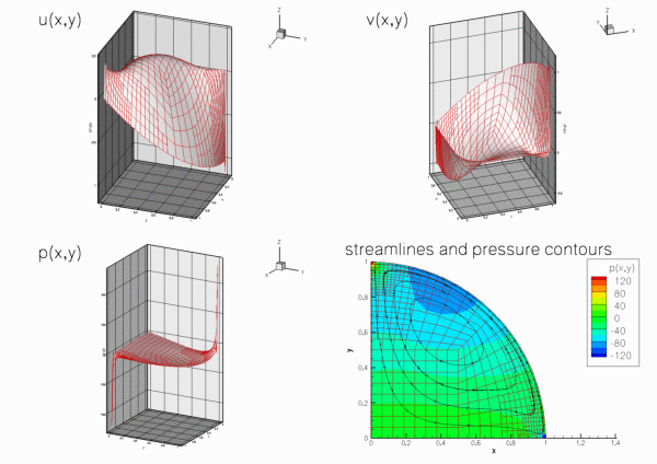
Try making the curved boundary the driving wall [Hint: this requires a change in the wall velocities prescribed in Problem::actions_before_newton_solve(). The figure below shows what you should expect.]

Plot of the velocity and pressure distribution for a circular driven cavity in which the flow is driven by the tangential motion of the curvilinear boundary.

Source files for this tutorial

The source files for this tutorial are located in the directory: demo_drivers/navier_stokes/circular_driven_cavity/
The driver code is: demo_drivers/navier_stokes/circular_driven_cavity/circular_driven_cavity.cc

PDF file

A pdf version of this document is available.