The aim of this tutorial is to demonstrate the solution of the time-harmonic equations of linear elasticity in cartesian coordinates. These equations are useful to describe forced, time-harmonic oscillations of elastic bodies.

Acknowledgement:

The implementation of the equations and the documentation were developed jointly with David Nigro.

Theory

Consider a linearly elastic body (of density $\rho$ , Young's modulus and Poisson's ratio $\nu$ ), occupying the region whose boundary is $\partial D$ . Assuming that the body performs time-harmonic oscillations of frequency of $\omega$ its motion is governed by the equations of time-harmonic linear elasticity

$\pmb{\nabla}^*\cdot\pmb{\tau}^*+ \rho \mathbf{F}^*=-\rho\omega^2 \mathbf{u}^*,$

where the $x_{i}^*$ are the cartesian coordinates, and the time-periodic stresses, body force and displacements are given by ${\rm Re}\{\pmb{\tau^*}(x_{i}^*){\rm e}^{-{\rm i}\omega t^*}\}$ , ${\rm Re}\{\mathbf{F}^*(x_{i}^*){\rm e}^{-{\rm i}\omega t^*}\}$ and ${\rm Re}\{\mathbf{u}^*(x_{i}^*){\rm e}^{-{\rm i}\omega t^*}\}$ respectively. Note that, as usual, the superscript asterisk notation is used to distinguish dimensional quantities from their non-dimensional counterparts where required.

The body is subject to imposed time-harmonic displacements ${\rm Re}\{\mathbf{\hat{u}}^* {\rm e}^{-{\rm i}\omega t^*}\}$ along $\partial D_d$ , and to an imposed time-harmonic traction ${\rm Re}\{ \pmb{\hat{\tau}}^* {\rm e}^{-{\rm i}\omega t^*}\}$ along $\partial D_n$ where $\partial D=\partial D_d\cup\partial D_n$ . This requires that

$\mathbf{u}^*=\mathbf{\hat{u}}^*\,\,\textrm{on $ \partial D_d $ },\quad \pmb{\tau}^* \cdot {\mathbf{n}}=\pmb{\hat{\tau}}^*\,\,\textrm{on $ \partial D_n $ }$

where ${\bf n}$ is the outer unit normal on the boundary.

The stresses and displacements are related by the constitutive equations

$\pmb{\tau}^*=\frac{E}{1+\nu}\left( \frac{\nu}{1-2\nu}(\pmb{\nabla}^*\cdot\mathbf{u}^*)\textbf{I}+ \frac{1}{2}(\pmb{\nabla}^*\mathbf{u}^*+\pmb{\nabla}^*\mathbf{u}^{*{\rm T}})\right),$

where $\pmb{\nabla}^*\mathbf{u}^{*{\rm T}}$ represents the transpose of $\pmb{\nabla}^*\mathbf{u}^*$ .

We non-dimensionalise the equations, using a problem specific reference length, ${\cal L}$ , and a timescale $\displaystyle {\cal T}=\frac{1}{\omega}$ , and use Young's modulus to non-dimensionalise the body force and the stress tensor:

$\pmb{\tau}^* = E \, \pmb{\tau}, \qquad x_{i}^* = {\cal L}\, x_{i}$

$\mathbf{u}^* = {\cal L}\, \mathbf{u}, \qquad \mathbf{F}^* = \frac{E}{\rho \cal L} \, \mathbf{F}, \qquad t^* = {\cal T}\, t.$

The non-dimensional form of the equations is then given by

$\pmb{\nabla}\cdot\pmb{\tau}+\mathbf{F}=-\Omega^2\mathbf{u}, \ \ \ \ \ \ \ \ \ \ (1)$

with the non-dimensional constitutive relation,

$\pmb{\tau}=\frac{1}{1+\nu}\left( \frac{\nu}{1-2\nu}(\pmb{\nabla}\cdot\mathbf{u})\textbf{I}+ \frac{1}{2}(\pmb{\nabla}\mathbf{u}+\pmb{\nabla}\mathbf{u}^{{\rm T}})\right). \ \ \ \ \ \ \ \ \ \ (2)$

The non-dimensional parameter

$\Omega = {\cal L}\omega \sqrt{\frac{\rho}{E}}$

is the ratio of the elastic body's intrinsic timescale, $\displaystyle {\cal L} \sqrt{\frac{\rho}{E}}$ , to the problem-specific timescale, $\displaystyle {\cal T}=\frac{1}{\omega}$ , that we used to non-dimensionalise time. $\Omega$ can be interpreted as a non-dimensional version of the excitation frequency; alternatively/equivalently $\Omega^2$ may be interpreted as a non-dimensional density. The boundary conditions are

$\mathbf{u}=\mathbf{\hat{u}}\,\,\textrm{on $\partial D_d $ },\quad \pmb{\tau} \cdot {\mathbf{n}}=\pmb{\hat{\tau}}\,\,\textrm{on $\partial D_n $ }.$

Implementation

Within oomph-lib, the non-dimensional version of equations (1) with the constitutive equations (2) are implemented in the TimeHarmonicLinearElasticityEquations<DIM> equations class, where the template parameter DIM indicates the spatial dimension. Following our usual approach, discussed in the (Not-So-)Quick Guide, this equation class is then combined with a geometric finite element to form a fully-functional finite element. For instance, the combination of the TimeHarmonicLinearElasticityEquations<2> class with the geometric finite element QElement<2,3> yields a nine-node quadrilateral element. As usual, the mapping between local and global (Eulerian) coordinates within an element is given by,

$x_i = \sum_{j=1}^{N^{(E)}} X^{(E)}_{ij} \, \psi_j, \qquad i=1,2,$

where $N^{(E)}$ is the number of nodes in the element, $X^{(E)}_{ij}$ is the -th global (Eulerian) coordinate of the -th Node in the element, and the $\psi_j$ are the element's shape functions, defined in the geometric finite element.

All the constitutive parameters are real. The two components of the displacement field have a real and imaginary part. We store the four real-valued nodal unknowns in the order ${\rm Re}\{u_x\}, {\rm Re}\{u_y\}, {\rm Im}\{u_x\}, {\rm Im}\{u_y\}$ and use the shape functions to interpolate the displacements as

$u_i^{(n)} = \sum_{j=1}^{N^{(E)}} U^{(E)}_{ij} \, \psi_j, \qquad i=1,...4,$

where $U^{(E)}_{ij}$ is the -th displacement component (enumerated as described above) at the -th Node in the element.

A test problem: Oscillations of an elastic annulus

We consider the time-harmonic axisymmetric deformation of a 2D annular elastic body that occupies the region $r_{\rm min}\leq r\leq r_{\rm max}, 0\leq\theta\leq 2\pi$ , shown in the left half of the sketch below. We impose a constant-amplitude axisymmetric displacement ${\mathbf{u}}(r_{\rm min},\theta)= u_0 (1-{\rm i}) {\mathbf{e}}_r$ on the inner boundary and a constant-amplitude pressure load $\pmb{\hat{\tau}} = -P_0 {\mathbf{e}}_r$ on the outer boundary. ( ${\mathbf{e}}_r$ is the unit vector in the radial direction).

Sketch of the test problems.

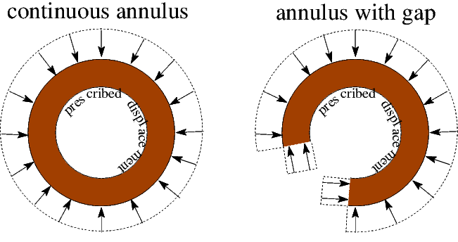
It is easy to find an analytical solution of this problem by working in polar coordinates and exploiting the axisymmetry of the solution by writing the displacement as $\displaystyle {\mathbf{u}} = U(r) {\mathbf{e}}_r$ . The radial displacement is then governed by

$\frac{d}{d r}\left(\frac{U}{r}+\frac{dU}{dr}\right) + k^2 U=0,$

where $\displaystyle k^2= \frac{\Omega^2}{\lambda+2\mu}$ and

$\lambda = \frac{\nu}{(1+\nu)(1-2\nu)} \qquad \textrm{and} \qquad \mu = \frac{1}{2(1+\nu)}$

are the non-dimensional Lame parameters. The solution of this equation is given by:

$U(r) = aJ_1(kr)+bY_1(kr).$

where and are Bessel functions of the first and second kind, respectively. The amplitudes and can be found using the boundary conditions on $r_{\rm min}$ and $r_{\rm max}$ . In the driver code discussed below, the (lengthy) expressions for and in terms of the problem parameters can be found in the GlobalParameters::exact_u() function.

We note that even though a relatively simple analytical solution (in polar coordinates!) exists for this problem, it is a non-trivial test case for our code which solves the governing equations in cartesian coordinates. However, to show that we can also compute non-trivial solutions, we also consider the case where the annular region has a "gap" and therefore occupies only a fraction (90%) of the circumference. This creates two additional boundaries (the radial lines bounding the "gap" and we subject these to the same pressure that acts on the outer boundary, as shown in the right half of the sketch above.

Results

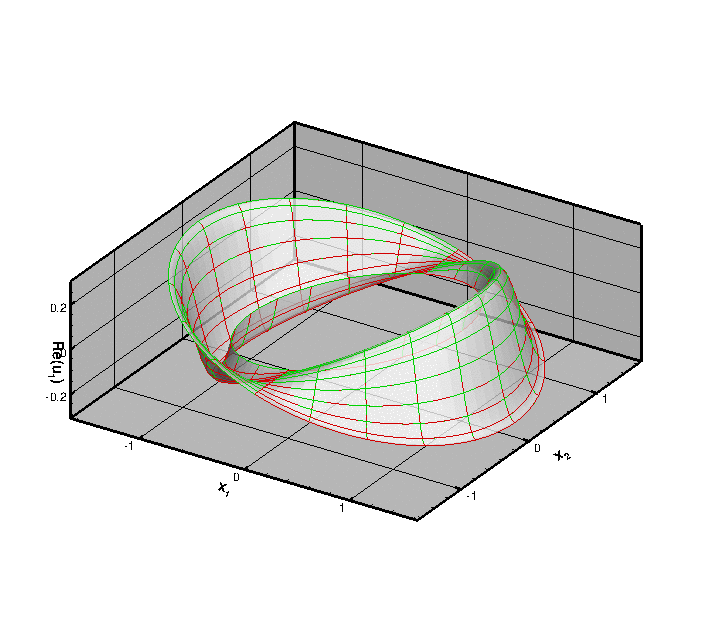
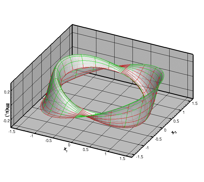
The figures below show "carpet plots" of the real and imaginary parts of the exact (green) and computed (red) horizontal displacement ( – the plots for obviously look very similar) for the continuous coating and $\Omega^2=10$ , $\nu=0.3$ , , $r_{\rm min}=1$ and $r_{\rm max}=1.5$ .

Real part of the horizontal displacement. Green: exact; red: computed.

Imaginary part of the horizontal displacement. Green: exact; red: computed.

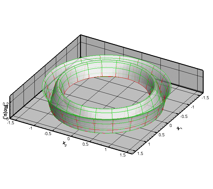
To demonstrate that the resulting displacement field is indeed axisymmetric, here is a plot of the real part of the radial displacement, $( Re(u_1)^2 + Re(u_2)^2 )^{1/2}$ .

Real part of the radial displacement. Green: exact; red: computed.

Finally, here is a plot of the real part of the horizontal displacement for the case when there is a 10% "gap" in the annular region. The presence of the gap clearly breaks the axisymmetry of the solution and creates waves that propagate in all directions:

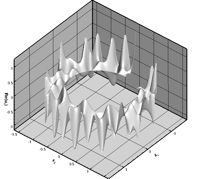
Real part of the horizontal displacement for an incomplete annular region.

Unsurprisingly, we are not aware of an analytical solution for this problem.

Global parameters and functions

As usual, we define all non-dimensional parameters in a namespace where we also define the displacement to be applied on the inner boundary, the traction (pressure) to be applied on the outer boundary, and the exact solution (which we don't list here because it is very lengthy).

//=======start_namespace==========================================
/// Global variables
//================================================================
namespace Global_Parameters
{
 
 /// Poisson's ratio
 double Nu = 0.3;
 
 /// Square of non-dim frequency
 double Omega_sq=100.0;
  
 /// The elasticity tensor
 TimeHarmonicIsotropicElasticityTensor E(Nu);
 
 /// Thickness of annulus
 double H_annulus=0.5;
 
 /// Displacement amplitude on inner radius
 double Displacement_amplitude=0.1;
 
 /// Real-valued, radial displacement field on inner boundary
 void solid_boundary_displacement(const Vector<double>& x,
                                  Vector<double>& u)
 {
  Vector<double> normal(2);
  double norm=sqrt(x[0]*x[0]+x[1]*x[1]);
  normal[0]=x[0]/norm;
  normal[1]=x[1]/norm;
 
  u[0]=Displacement_amplitude*normal[0];
  u[1]=Displacement_amplitude*normal[1];
 }
 
 /// Uniform pressure
 double P = 0.0;
 
 /// Constant pressure load (real and imag part)
 void constant_pressure(const Vector<double> &x,
                        const Vector<double> &n, 
                        Vector<std::complex<double> >&traction)
 {
  unsigned dim = traction.size();
  for(unsigned i=0;i<dim;i++)
   {
    traction[i] = complex<double>(-P*n[i],P*n[i]);
   }
 } // end_of_pressure_load

We also define the output directory and the number of elements in the mesh.

 /// Output directory
 string Directory="RESLT";
 
 /// Number of elements in azimuthal direction 
 unsigned Ntheta=20;
 
 /// Number of elements in radial direction 
 unsigned Nr=10;

The driver code

We start by defining command line arguments which specify the number of elements in the mesh and indicate the presence or absence of the "gap" in the coating.

//=======start_of_main==================================================
/// Driver for annular disk loaded by pressure
//======================================================================
int main(int argc, char **argv)
{
 
 // Store command line arguments
 CommandLineArgs::setup(argc,argv);
 
 // Define possible command line arguments and parse the ones that
 // were actually specified
 
 // Number of elements in azimuthal direction
 CommandLineArgs::specify_command_line_flag(
  "--ntheta",
  &Global_Parameters::Ntheta);
 
 // Number of elements in radial direction
 CommandLineArgs::specify_command_line_flag(
  "--nr",
  &Global_Parameters::Nr);
 
 // Do have a gap in the annulus?
 CommandLineArgs::specify_command_line_flag("--have_gap");

The code performs a parameter study in which we compute the solution for a range of pressures. We specify the pressure increment and the number of steps to be performed, parse the command line arguments and document them.

 // P increment
 double p_increment=0.1;
 CommandLineArgs::specify_command_line_flag("--p_increment",&p_increment);
 
 // Number of steps
 unsigned nstep=3; 
 CommandLineArgs::specify_command_line_flag("--nstep",&nstep);
 
 // Parse command line
 CommandLineArgs::parse_and_assign(); 
 
 // Doc what has actually been specified on the command line
 CommandLineArgs::doc_specified_flags();

Next, we create the problem (discretising the domain with nine-noded quadrilateral elements),

//Set up the problem

AnnularDiskProblem<RefineableQTimeHarmonicLinearElasticityElement<2,3> >

AnnularDiskProblem

Annular disk.

Definition: time_harmonic_elastic_annulus.cc:301

and perform the parameter study:

 // Initial values for parameter values
 Global_Parameters::P=0.0; 
 
 //Parameter incrementation
 for(unsigned i=0;i<nstep;i++)
  {
   // Solve the problem using Newton's method
   problem.newton_solve();
   // Doc solution
   problem.doc_solution();
   
   // Increment pressure
   Global_Parameters::P+=p_increment;
  }
 
} //end of main

The problem class

The Problem class is very simple. As in other problems with Neumann boundary conditions, we provide separate meshes for the "bulk" elements and the face elements that apply the traction boundary conditions. The latter are attached to the relevant faces of the bulk elements by the function create_traction_elements().

//=============begin_problem============================================ 
/// Annular disk
//====================================================================== 
template<class ELASTICITY_ELEMENT>
class AnnularDiskProblem : public Problem
{
 
public:
 
 /// Constructor:
 AnnularDiskProblem();
 
 /// Update function (empty)
 void actions_after_newton_solve() {}
 
 /// Update function (empty)
 void actions_before_newton_solve() {}
 /// Doc the solution
 void doc_solution();
 
private:
 
 /// Create traction elements
 void create_traction_elements();
 
 /// Delete traction elements
 void delete_traction_elements();
 /// Pointer to solid mesh
 Mesh* Solid_mesh_pt;
 /// Pointer to mesh of traction elements
 Mesh* Traction_mesh_pt;
 
 /// DocInfo object for output
 DocInfo Doc_info;
 
};

The problem constructor

We begin by building the "bulk" solid mesh, specifying the presence of the gap (and its width) if necessary. If there is no gap, the mesh is periodic; see Comments for a more detailed discussion of how the mesh for this problem is constructed.

//===========start_of_constructor======================================= 
/// Constructor: 
//====================================================================== 
template<class ELASTICITY_ELEMENT>
AnnularDiskProblem<ELASTICITY_ELEMENT>::AnnularDiskProblem() 
{
 
 // Solid mesh
 //-----------
 
 // The mesh is periodic 
 bool periodic=true;
 
 // Azimuthal fraction of elastic coating
 double azimuthal_fraction_of_coating=1.0;
 
 // Innermost radius for solid mesh
 double a=1.0;
 
 // Gap in annulus?
 if (CommandLineArgs::command_line_flag_has_been_set("--have_gap"))
  {
   periodic=false;
   azimuthal_fraction_of_coating=0.9;
  }
 // Build solid mesh
 Solid_mesh_pt = new 
  RefineableTwoDAnnularMesh<ELASTICITY_ELEMENT>(
   periodic,azimuthal_fraction_of_coating,
   Global_Parameters::Ntheta,
   Global_Parameters::Nr,a,
   Global_Parameters::H_annulus);

It is always a good idea to have a look at the mesh and its boundary enumeration:

 // Let's have a look where the boundaries are
 Solid_mesh_pt->output("solid_mesh.dat");
 Solid_mesh_pt->output_boundaries("solid_mesh_boundary.dat");

We loop over the elements and specify the relevant physical parameters via the pointer to the tensor of constitutive parameters and the (square of the) non-dimensional frequency,

 
 
 //Assign the physical properties to the elements
 //Loop over the elements in the main mesh
 unsigned n_element =Solid_mesh_pt->nelement();
 for(unsigned i=0;i<n_element;i++)
  {
   //Cast to a solid element
   ELASTICITY_ELEMENT *el_pt = 
    dynamic_cast<ELASTICITY_ELEMENT*>(Solid_mesh_pt->element_pt(i));
   
   // Set the constitutive law
   el_pt->elasticity_tensor_pt() = &Global_Parameters::E;
 
   // Square of non-dim frequency
   el_pt->omega_sq_pt()= &Global_Parameters::Omega_sq;
  }

Next we create the mesh that contains the FaceElements that apply the traction boundary conditions, and combine all meshes into a global mesh:

 
 // Construct the traction element mesh
 Traction_mesh_pt=new Mesh;
 create_traction_elements(); 
 
 // Solid mesh is first sub-mesh
 add_sub_mesh(Solid_mesh_pt);
 
 // Add traction sub-mesh
 add_sub_mesh(Traction_mesh_pt);
 
 // Build combined "global" mesh
 build_global_mesh();

We apply the displacement boundary conditions by pinning the real and imaginary part of the two displacement components at all nodes on boundary 0. We then impose a purely radial displacement on the real and imaginary parts of the displacement field, using the function defined in the Global_Parameters namespace:

 // Solid boundary conditions:
 //---------------------------
 
 // Pin real and imag part of both displacement components 
 // on the inner (boundary 0)
 unsigned b_inner=0;
 unsigned n_node = Solid_mesh_pt->nboundary_node(b_inner);
 
 //Loop over the nodes to pin and assign boundary displacements on 
 //solid boundary
 Vector<double> u(2);
 Vector<double> x(2);
 for(unsigned i=0;i<n_node;i++)
  {
   Node* nod_pt=Solid_mesh_pt->boundary_node_pt(b_inner,i);
   nod_pt->pin(0);
   nod_pt->pin(1);
   nod_pt->pin(2);
   nod_pt->pin(3);
   
   // Assign displacements
   x[0]=nod_pt->x(0);   
   x[1]=nod_pt->x(1);   
   Global_Parameters::solid_boundary_displacement(x,u);
 
   // Real part of x-displacement
   nod_pt->set_value(0,u[0]);
   // Real part of y-displacement
   nod_pt->set_value(1,u[1]);
   // Imag part of x-displacement
   nod_pt->set_value(2,-u[0]);
   // Imag part of y-displacement
   nod_pt->set_value(3,-u[1]);
  }

Finally we assign the equation numbers and specify the output directory:

 
 //Assign equation numbers
 cout << assign_eqn_numbers() << std::endl; 
 
 // Set output directory
 Doc_info.set_directory(Global_Parameters::Directory);
 
} //end_of_constructor

The traction elements

We create the face elements that apply the traction on the outer boundary (boundary 2). If there is a gap in the annular region we also apply the pressure loading on boundaries 1 and 3.

//============start_of_create_traction_elements==============================
/// Create traction elements 
//=======================================================================
template<class ELASTICITY_ELEMENT>
void AnnularDiskProblem<ELASTICITY_ELEMENT>::create_traction_elements()
{
 
 // Load outer surface (2) and both "ends" (1 and 3) if there's a gap
 unsigned b_lo=1;
 unsigned b_hi=3;
 
 // ...otherwise load only the outside (2)
 if (!CommandLineArgs::command_line_flag_has_been_set("--have_gap"))
  {     
   b_lo=2;
   b_hi=2;
  }
 
 for (unsigned b=b_lo;b<=b_hi;b++)
  {
   // How many bulk elements are adjacent to boundary b?
   unsigned n_element = Solid_mesh_pt->nboundary_element(b);
   
   // Loop over the bulk elements adjacent to boundary b
   for(unsigned e=0;e<n_element;e++)
    {
     // Get pointer to the bulk element that is adjacent to boundary b
     ELASTICITY_ELEMENT* bulk_elem_pt = dynamic_cast<ELASTICITY_ELEMENT*>(
      Solid_mesh_pt->boundary_element_pt(b,e));
     
     //Find the index of the face of element e along boundary b
     int face_index = Solid_mesh_pt->face_index_at_boundary(b,e);
     
     // Create element
     TimeHarmonicLinearElasticityTractionElement<ELASTICITY_ELEMENT>* el_pt=
      new TimeHarmonicLinearElasticityTractionElement<ELASTICITY_ELEMENT>
      (bulk_elem_pt,face_index);   
 
     // Add to mesh
     Traction_mesh_pt->add_element_pt(el_pt);
     
     // Associate element with bulk boundary (to allow it to access
     // the boundary coordinates in the bulk mesh)
     el_pt->set_boundary_number_in_bulk_mesh(b); 
     
     //Set the traction function
     el_pt->traction_fct_pt() = Global_Parameters::constant_pressure;
    }
  }
 
} // end_of_create_traction_elements

Post-processing

As expected, this member function documents the computed solution.

//==============start_doc===========================================
/// Doc the solution
//==================================================================
template<class ELASTICITY_ELEMENT>
void AnnularDiskProblem<ELASTICITY_ELEMENT>::doc_solution()
{
 
 ofstream some_file;
 char filename[100];
 
 // Number of plot points
 unsigned n_plot=5; 
 
 // Output displacement field
 //--------------------------
 sprintf(filename,"%s/elast_soln%i.dat",Doc_info.directory().c_str(),
         Doc_info.number());
 some_file.open(filename);
 Solid_mesh_pt->output(some_file,n_plot);
 some_file.close();
 
 
 // Output traction elements
 //-------------------------
 sprintf(filename,"%s/traction_soln%i.dat",Doc_info.directory().c_str(),
         Doc_info.number());
 some_file.open(filename);
 Traction_mesh_pt->output(some_file,n_plot);
 some_file.close();
 
 // Output exact solution 
 //----------------------
 sprintf(filename,"%s/exact_soln%i.dat",Doc_info.directory().c_str(),
         Doc_info.number());
 some_file.open(filename);
 Solid_mesh_pt->output_fct(some_file,n_plot,Global_Parameters::exact_u); 
 some_file.close();
 
 // Increment label for output files
 Doc_info.number()++;
 
} //end doc

Comments and Exercises

Comments

We did not discuss the mesh generation in detail here: The mesh is created by straightforward overloading of oomph-lib's existing rectangular quad mesh – the constructor simply adjusts the nodal positions (exactly as suggested in the "Not-so-quick" guide.) A little bit of extra work is required to enforce periodicity on the mesh for the case without a gap in the annular region because two of the boundaries in the original mesh then overlap. How this is dealt with is discussed in another tutorial.
If you inspect the driver code you will notice that it also contains relevant code to perform spatially adaptive simulations of the problem – the adaptive version of the code is selected with #ifdefs. Dealing with the periodic boundary conditions for spatially adaptive meshes requires a few additional steps, but they are also discussed elsewhere, so we won't discuss them here.

Exercises

Change the parameter study performed by the driver code such that the loop varies the frequency parameter $\Omega^2$ . Assess the effect of an increase in $\Omega^2$ on the accuracy of the solution by comparing the computed results against the exact solution at fixed spatial resolution.
Explore the use of spatial adaptivity in the problem
- for the same parameter study suggested in the previous exercise (increase in $\Omega^2$ )

and

for the problem with the "gap" in the annular region.

Modify the code to exploit at least some of the problem's symmetry, e.g. by solving the problem for the continuous annulus in a quarter of the original domain, $x_1, x_2 \ge 0$ , say, using appropriate symmetry boundary conditions along the coordinate axes.

Source files for this tutorial

The source files for this tutorial are located in the directory: demo_drivers/time_harmonic_linear_elasticity/elastic_annulus
The driver code is: demo_drivers/time_harmonic_linear_elasticity/elastic_annulus/time_harmonic_elastic_annulus.cc

PDF file

A pdf version of this document is available.