In this tutorial we re-visit a linear elasticity problem that we already discussed in detail in another tutorial: The deformation of an elastic strip loaded by a periodic surface traction. We demonstrate how to solve the problem with spatial adaptivity and explain how to apply periodic boundary conditions in such problems.

The example problem

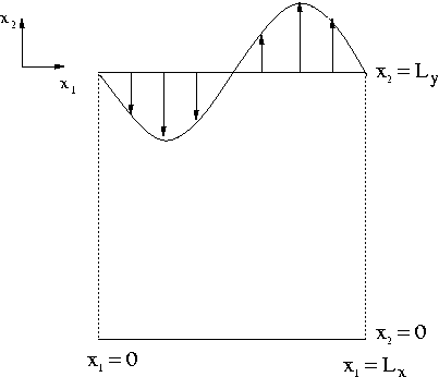
We consider the same problem that we discussed in another tutorial:

The problem.

Infinitely long strip loaded by a periodic traction.

Solve

$\frac{\partial \tau_{ij}}{\partial x_j} + F_i=0, \ \ \ \ \ \ \ \ \ \ (1)$

in the domain $D = \{x_1 \in [-\infty,+\infty], x_2 \in [0,L_y]\}$ , subject to the Dirichlet boundary conditions

$\left. \mathbf{u}\right|_{x_2 = 0}=(0,0), \ \ \ \ \ \ \ \ \ \ (2)$

on the bottom boundary, the Neumann (traction) boundary conditions

$\left. \mathbf{t}\right|_{x_2 = L_y}=\left(-A \cos{\left(\frac{2 \pi x_1}{L_x}\right)}, -A \sin{\left(\frac{2 \pi x_1}{L_x}\right)}\right), \ \ \ \ \ \ \ \ \ \ (3)$

on the top boundary, and symmetry conditions at

and

$\left. {\bf u}\right|_{x_1=0} = \left.{\bf u}\right|_{x_1=L_x}. \ \ \ \ \ \ \ \ \ \ (4)$

As before, we only discretise the domain over one period of the applied spatially-periodic traction and apply symmetry conditions at the left and right domain boundaries. Here we compute the solution with spatial adaptivity.

Results

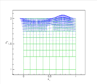
The figure below shows a vector plot of the displacement field near the upper domain boundary. As already observed in the computations with a spatially uniform discretisation, the displacements decay rapidly with distance from the loaded surface. oomph-lib's automatic mesh adaptation therefore chooses a much finer discretisation near the upper domain boundary than in the interior, leading to a significant reduction in the number of unknowns in the problem.

Plot of displacement field, computed with spatial adaptivity. Note that the mesh is much finer near the top boundary where the displacement (gradients) are large.

The driver code

Most of the driver code is identical to that discussed in the tutorial in which we solved the problem without spatial adaptivity. We will therefore only discuss the parts of the code that require significant changes.

The problem class

The problem class is very similar to that used in the non-refineable version of the problem. As usual, we detach the face elements that apply the traction boundary condition before adapting the bulk mesh and then re-attach them afterwards. This is done by the functions delete_traction_elements() and assign_traction_elements() which are called from actions_before_adapt() and actions_after_adapt(), respectively.

//===start_of_problem_class=============================================
/// Periodic loading problem
//======================================================================
template<class ELEMENT>
class RefineablePeriodicLoadProblem : public Problem
{
public:
 
 /// Constructor: Pass number of elements in x and y directions 
 /// and lengths.
 RefineablePeriodicLoadProblem(const unsigned &nx, const unsigned &ny, 
                               const double &lx, const double &ly);
 
 /// Update before solve is empty
 void actions_before_newton_solve() {}
 
 /// Update after solve is empty
 void actions_after_newton_solve() {}
 
 /// Actions before adapt: Wipe the mesh of traction elements
 void actions_before_adapt()
  {
   // Kill the traction elements and wipe surface mesh
   delete_traction_elements();
   
   // Rebuild the Problem's global mesh from its various sub-meshes
   rebuild_global_mesh();
  }
 
 /// Actions after adapt: Rebuild the mesh of traction elements
 void actions_after_adapt()
  {
   // Create traction elements
   assign_traction_elements();
 
   // Rebuild the Problem's global mesh from its various sub-meshes
   rebuild_global_mesh();
  }
 
 /// Doc the solution
 void doc_solution(DocInfo& doc_info);
 
private:
 
 /// Allocate traction elements on the top surface
 void assign_traction_elements();
 
 /// Kill traction elements on the top surface
 void delete_traction_elements()
  {
   // How many surface elements are in the surface mesh
   unsigned n_element = Surface_mesh_pt->nelement();
   
   // Loop over the traction elements
   for(unsigned e=0;e<n_element;e++)
    {
     // Kill surface element
     delete Surface_mesh_pt->element_pt(e);
    }
   
   // Wipe the mesh
   Surface_mesh_pt->flush_element_and_node_storage();
  }
 
 /// Pointer to the (refineable!) bulk mesh
 TreeBasedRefineableMeshBase* Bulk_mesh_pt;
 
 /// Pointer to the mesh of traction elements
 Mesh* Surface_mesh_pt;
 
}; // end_of_problem_class

The problem constructor – applying periodic boundary condition in spatially adaptive computations.

A key feature of this problem is the presence of the periodic boundary conditions (4) which require that the displacement field at the left boundary is the same as that on the right one. As discussed in another tutorial, such constraints can be imposed by the function

BoundaryNode::make_periodic(...).

Once this function is called for a BoundaryNode, the BoundaryNode shares its Data with the Node specified as the argument to that function. This "wraps the solution around the domain".

In spatially adaptive computations a complication arises because the non-uniform refinement of a mesh creates so-called hanging nodes, i.e. nodes in a refined element that have no counterpart in an adjacent less-refined element. Within oomph-lib, such hanging nodes
are automatically constrained to maintain the inter-element continuity of the solution. The automatic detection of hanging nodes requires the identification of the elements' neighbours. This task is performed by neighbour finding routines that operate on a tree-(forest-)based representation of a mesh's refinement pattern; see the discussion in
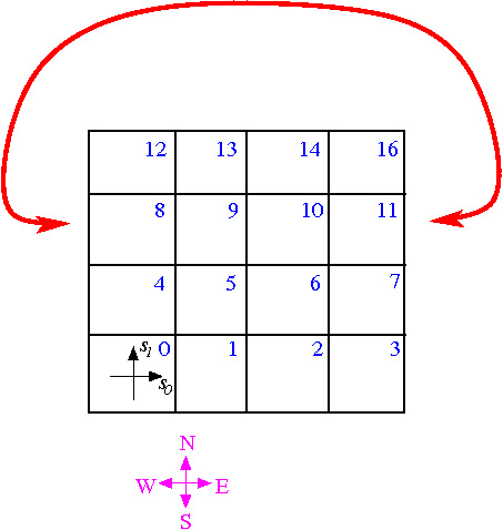
the tutorial explaining oomph-lib's overall data structure. The representation of the initial, unrefined mesh as a TreeForest, required by these routines, is typically generated in the mesh constructor, using the function TreeBasedRefineableMeshBase::setup_tree_forest(). In the 4x4 mesh shown below this function would establish that within the Forest representing this mesh, the Tree associated with element 11 has three neighbours: Element 16 in the northern (N) direction; element 10 in the western (W) direction; element 7 in the southern (S) direction. There is no neighbour in the eastern (E) direction. If element 11 is refined but its neighbours are not, the hanging nodes on the edges with elements 7, 10 and 16 are automatically detected and constrained, maintaining the continuity of the solution across the element boundaries.

Sketch illustrating neighbour finding in problems with periodic boundary conditions.

If periodic boundary conditions are applied, the "wrapping around" of the domain (indicated by the red line) means that element 8 must be regarded as the (periodic) eastern (E) neighbour of element 11. This information must be passed to the root of the Tree associated with element 11, using the functions TreeRoot::neighbour_pt(...) and TreeRoot::neighbour_periodic(...).

This is illustrated in the following code segment which shows the revised version of the problem constructor. We start by building the refineable mesh and set the spatial error estimator.

//===start_of_constructor=============================================
/// Problem constructor: Pass number of elements in the coordinate
/// directions and the domain sizes.
//====================================================================
template<class ELEMENT>
RefineablePeriodicLoadProblem<ELEMENT>::RefineablePeriodicLoadProblem
(const unsigned &nx, const unsigned &ny,
 const double &lx, const double& ly)
{
 // Create the mesh 
 Bulk_mesh_pt = new RefineableRectangularQuadMesh<ELEMENT>(nx,ny,lx,ly);
 
 // Create/set error estimator
 Bulk_mesh_pt->spatial_error_estimator_pt()=new Z2ErrorEstimator;

Next we declare all nodes on boundary 1 (the right boundary) to be periodic counterparts of the corresponding nodes on boundary 3 (the left boundary). (Here we exploit that within this particular mesh the boundary nodes on the left and right boundaries are enumerated consistently from top to bottom; this is not guaranteed to be the case – for a general mesh you will have to establish which node corresponds to which; see Comments and Exercises .)

 
 // Make the mesh periodic in the x-direction by setting the nodes on
 // right boundary (boundary 1) to be the periodic counterparts of
 // those on the left one (boundary 3).
 unsigned n_node = Bulk_mesh_pt->nboundary_node(1);
 for(unsigned n=0;n<n_node;n++)
  {
   Bulk_mesh_pt->boundary_node_pt(1,n)
    ->make_periodic(Bulk_mesh_pt->boundary_node_pt(3,n));
  }

We obtain the tree roots associated with the elements on the left and right boundaries, again exploiting the specific enumeration of the elements (from bottom left to top right, as in the sketch shown above).

 
 
 // Now establish the new neighbours (created by "wrapping around"
 // the domain) in the TreeForst representation of the mesh
 
 // Get pointers to tree roots associated with elements on the 
 // left and right boundaries
  Vector<TreeRoot*> left_root_pt(ny);
  Vector<TreeRoot*> right_root_pt(ny);
  for(unsigned i=0;i<ny;i++) 
   {
    left_root_pt[i] = 
     dynamic_cast<ELEMENT*>(Bulk_mesh_pt->element_pt(i*nx))->
     tree_pt()->root_pt();
    right_root_pt[i] = 
     dynamic_cast<ELEMENT*>(Bulk_mesh_pt->element_pt(nx-1+i*nx))->
     tree_pt()->root_pt();
   }

Using this information it is easy to establish the (periodic) connections between the trees:

 
  // Switch on QuadTreeNames for enumeration of directions
   using namespace QuadTreeNames;
 
  //Set the neighbour and periodicity
  for(unsigned i=0;i<ny;i++) 
   {
    // The western neighbours of the elements on the left
    // boundary are those on the right
    left_root_pt[i]->neighbour_pt(W) = right_root_pt[i];
    left_root_pt[i]->set_neighbour_periodic(W); 
    
    // The eastern neighbours of the elements on the right
    // boundary are those on the left
    right_root_pt[i]->neighbour_pt(E) = left_root_pt[i];
    right_root_pt[i]->set_neighbour_periodic(E);     
   } // done

The rest of the problem constructor is identical to that in its non-refineable counterpart and is therefore omitted here.

Comments and Exercises

Comments

When setting up periodic boundary conditions, it is obviously important to correctly identify the corresponding nodes and elements on the mesh boundaries. The enumeration of these nodes and elements is typically performed in the mesh constructor. If you are unsure what conventions have been used (and are too lazy to read the source code), recall that you can use the function

Mesh::boundary_node_pt(b,j)

to obtain a pointer to the j -th node on the Mesh's b -th boundary and

Mesh::boundary_element_pt(b,j)

to obtain a pointer to the j -th element on the Mesh's b -th boundary.

Exercises

Modify the problem constructor to check that the vertical coordinate of each periodic node matches that of its non-periodic counterpart.
Confirm that the computed solution has a small discontinuity across the periodic boundary when you
1. comment out the assignment of the periodic tree neighbours
2. force the refinement of a single element next to the left boundary, say.

The relevant code is for the latter task is, in fact, already implemented in the problem constructor because the driver code acts as a self-test for this functionality.

 // Do selective refinement of one element so that we can test
 // whether periodic hanging nodes work: Choose a single element 
 // (the zero-th one) as the to-be-refined element.
 // This creates a hanging node on the periodic boundary
 Vector<unsigned> refine_pattern(1,0);
 Bulk_mesh_pt->refine_selected_elements(refine_pattern);

Note: To facilitate the visualisation of the discontinuity it is helpful to perform this test with the bilinear RefineableQLinearElasticityElement<2,2>, with a shallower domain (e.g. ), and without any further spatial refinement (set max_adapt=0 in main() ).

Source files for this tutorial

The source files for this tutorial are located in the directory: demo_drivers/linear_elasticity/periodic_load/
The driver code is: demo_drivers/linear_elasticity/periodic_load/refineable_periodic_load.cc

PDF file

A pdf version of this document is available.