This is our first linear elasticity example problem. We discuss the non-dimensionalisation of the governing equations and their implementation in oomph-lib, and then demonstrate the solution of a 2D problem: the deformation of an elastic strip by a periodic traction.

Acknowledgement: This tutorial and the associated driver code was developed jointly with David Rutter.

The governing equations

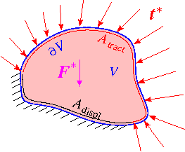
The figure below shows a sketch of a general elasticity problem. A linearly elastic solid body occupies the domain and is loaded by a body force ${\bf F}^*$ and by a surface traction ${\bf t}^*$ which is applied along part of its boundary, $A_{\rm tract}$ . The displacement is prescribed along the remainder of the boundary, $A_{\rm displ}$ , where $\partial V = A_{\rm tract} \cup A_{\rm displ}$ .

Sketch of a general elasticity problem: A linearly elastic body is loaded by a body force and is exposed to a prescribed traction along part of its boundary while the displacement is prescribed along the remainder of the boundary.

We adopt an Eulerian approach and describe the deformation in terms of the displacement field ${\bf u}^*\left( x_i^*,t^* \right)$ where and are the spatial coordinates and time, respectively. Throughout this document we will use index notation and the summation convention, and use asterisks to distinguish dimensional quantities from their non-dimensional counterparts.
Denoting the density of the body by $\rho$ , the deformation is governed by the Cauchy equations,

$\frac{\partial \tau_{ij}^*}{\partial x_j^*} + \rho F_i^* = \rho \frac{\partial^2 u_i^*}{\partial t^{2*}},$

where $\tau_{ij}^*$ is the Cauchy stress tensor which, for a linearly elastic solid, is given by

$\tau_{ij}^* = E_{ijkl}^* \ e_{kl},$

where $e_{kl}$ is the strain tensor,

$e_{ij} = \frac{1}{2} \left( \frac{\partial u_i^*}{\partial x_j^*}+ \frac{\partial u_j^*}{\partial x_i^*}\right).$

$E_{ijkl}$ is the 4th order elasticity tensor, which for a homogeneous and isotropic solid is

$E_{ijkl}^* = \frac{E}{1+\nu} \left(\frac{\nu}{1-2\nu} \delta_{ij} \delta_{kl} + \delta_{ik} \delta_{jl} \right),$

where is Young's modulus, $\nu$ is the Poisson ratio and $\delta_{ij}$ is the Kronecker delta. Thus the Cauchy stress is given in terms of the displacement derivatives by

$\tau_{ij}^* = \frac{E}{1+\nu} \left(\frac{\nu}{1-2\nu} \ \delta_{ij} \ \frac{\partial u_k^*}{\partial x_k^*} + \frac{1}{2}\left(\frac{\partial u_i^*}{\partial x_j^*}+ \frac{\partial u_j^*}{\partial x_i^*} \right) \right).$

We non-dimensionalise the equations, using a problem specific reference length, ${\cal L}$ , and a timescale ${\cal T}$ , and use Young's modulus to non-dimensionalise the body force and the stress,

$\tau_{ij}^* = E \, \tau_{ij}, \qquad x_i^* = {\cal L}\, x_i, \qquad u_i^* = {\cal L}\, u_i,$

$t^* = {\cal T}\, t, \qquad F_i^* = \frac{E}{\rho \cal L} \, F_i. \qquad$

The non-dimensional form of the Cauchy equations is then given by

$\frac{\partial \tau_{ij}}{\partial x_j} + F_i = \Lambda^2 \frac{\partial^2 u_i}{\partial t^2}, \ \ \ \ \ \ \ \ \ \ (1)$

where

$\tau_{ij} = \frac{1}{1+\nu} \left(\frac{\nu}{1-2\nu} \ \delta_{ij} \ \frac{\partial u_k}{\partial x_k} + \frac{1}{2} \left(\frac{\partial u_i}{\partial x_j}+ \frac{\partial u_j}{\partial x_i} \right) \right). \ \ \ \ \ \ \ \ \ \ (2)$

The parameter

$\Lambda = \frac{{\cal L} \sqrt{\frac{\rho}{E}} }{\cal T},$

is the ratio of the elastic body's intrinsic timescale, ${\cal L} \sqrt{\frac{\rho}{E}}$ , to the problem-specific timescale, ${\cal T}$ , that we used to non-dimensionalise time.

The displacement constraints provide a Dirichlet condition for the displacements,

$u_i = u_i^{[\rm prescribed]} \ \ \ \ \ \ \mbox{on $A_{\mathrm{displ}}$},$

while the traction boundary conditions require that

$t_i = \tau_{ij} n_j \ \ \ \ \ \ \mbox{on $A_{\mathrm{tract}},$}$

where the are the components of the outer unit normal to the boundary.

In this tutorial we only consider steady problems for which the equations reduce to

$\frac{\partial \tau_{ij}}{\partial x_j} + F_i = 0.$

Implementation

The elements

Within oomph-lib, the non-dimensional version of the DIM-dimensional Cauchy equations (1) with the constitutive equations (2) are implemented in the LinearElasticityEquations<DIM> equations class. Following our usual approach, discussed in the (Not-So-)Quick Guide, this equation class is then combined with a geometric finite element to form a fully-functional finite element. For instance, the combination of the LinearElasticityEquations<2> class with the geometric finite element QElement<2,3> yields a nine-node quadrilateral linear elasticity element. As usual, the mapping between local and global (Eulerian) coordinates within an element is given by,

$x_i = \sum_{j=1}^{N^{(E)}} X^{(E)}_{ij} \, \psi_j, \qquad i=1,2\quad [\mbox{and }3],$

where $N^{(E)}$ is the number of nodes in the element, $X^{(E)}_{ij}$ is the -th global (Eulerian) coordinate of the -th Node in the element, and the $\psi_j$ are the element's shape functions, defined in the geometric finite element.

The cartesian displacement components
[and ] are stored as nodal values, and the shape functions are used to interpolate the displacements as

$u_i = \sum_{j=1}^{N^{(E)}} U^{(E)}_{ij} \, \psi_j, \qquad i=1,2\quad [\mbox{and }3],$

where $U^{(E)}_{ij}$ is the -th displacement component at the -th Node in the element. Nodal values of the displacement components are accessible via the access function

LinearElasticityEquations<DIM>::u(i,j)

which returns the -th displacement component stored at the element's -th Node.

The example problem

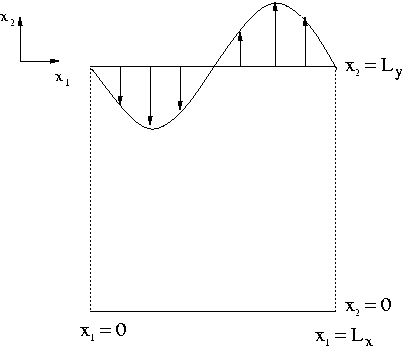
To illustrate the solution of the steady equations of linear elasticity, we consider the 2D problem shown in the sketch below.

The problem.

Infinitely long strip loaded by a periodic traction.

Solve

$\frac{\partial \tau_{ij}}{\partial x_j} + F_i=0, \ \ \ \ \ \ \ \ \ \ (3)$

in the domain $D = \{x_1 \in [-\infty,+\infty], x_2 \in [0,L_y]\}$ , subject to the Dirichlet boundary conditions

$\left. \mathbf{u}\right|_{x_2 = 0}=(0,0), \ \ \ \ \ \ \ \ \ \ (4)$

on the bottom boundary, the Neumann (traction) boundary conditions

$\left. \mathbf{t}\right|_{x_2 = L_y}=\left(-A \cos{\left(\frac{2 \pi x_1}{L_x}\right)}, -A \sin{\left(\frac{2 \pi x_1}{L_x}\right)}\right), \ \ \ \ \ \ \ \ \ \ (5)$

on the top boundary, and symmetry conditions at

and

$\left. {\bf u}\right|_{x_1=0} = \left.{\bf u}\right|_{x_1=L_x}.$

We note that for $L_y \to \infty$ the problem converges to the analytical solution.

$u_1^{[exact]} = -\frac{A(1+\nu)}{2 \pi} \cos{\left(\frac{2 \pi x_1}{L_x}\right)} \exp{\left(2 \pi (x_2-L_y)\right)},$

$u_2^{[exact]} = -\frac{A(1+\nu)}{2 \pi} \sin{\left(\frac{2 \pi x_1}{L_x}\right)} \exp{\left(2 \pi (x_2-L_y)\right)},$

Results

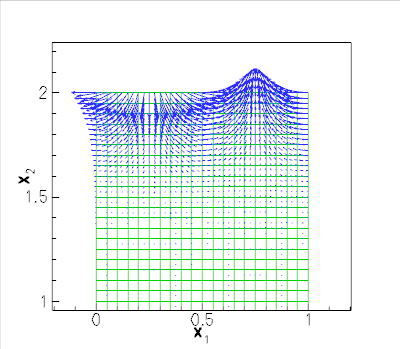
The figure below shows a vector plot of the displacement field near the upper domain boundary for and .
Note that we only discretised the infinite strip over one period of the applied, spatially-periodic surface traction, and imposed symmetry conditions on the left and right mesh boundaries.

The plot shows that the displacements decay rapidly with distance from the loaded surface – as suggested by the analytical solution for the infinite depth case. This suggests that the computation could greatly benefit from the use of spatial adaptivity. This is indeed the case and is explored in another tutorial.

Plot of the displacement field.

Global parameters and functions

As usual, we define all non-dimensional parameters in a namespace.

//===start_of_namespace=================================================
/// Namespace for global parameters
//======================================================================
namespace Global_Parameters
{
 /// Amplitude of traction applied
 double Amplitude = 1.0;
 
 /// Specify problem to be solved (boundary conditons for finite or
 /// infinite domain).
 bool Finite=false;
 
 /// Define Poisson coefficient Nu
 double Nu = 0.3;
 
 /// Length of domain in x direction
 double Lx = 1.0;
 
 /// Length of domain in y direction
 double Ly = 2.0;
 
 /// The elasticity tensor
 IsotropicElasticityTensor E(Nu);
 
 /// The exact solution for infinite depth case
 void exact_solution(const Vector<double> &x,
                     Vector<double> &u)
 {
  u[0] = -Amplitude*cos(2.0*MathematicalConstants::Pi*x[0]/Lx)*
        exp(2.0*MathematicalConstants::Pi*(x[1]-Ly))/
        (2.0/(1.0+Nu)*MathematicalConstants::Pi);
  u[1] = -Amplitude*sin(2.0*MathematicalConstants::Pi*x[0]/Lx)*
        exp(2.0*MathematicalConstants::Pi*(x[1]-Ly))/
        (2.0/(1.0+Nu)*MathematicalConstants::Pi);
 }
 
 /// The traction function
void periodic_traction(const double &time,
                       const Vector<double> &x,
                       const Vector<double> &n,
                       Vector<double> &result)
 {
  result[0] = -Amplitude*cos(2.0*MathematicalConstants::Pi*x[0]/Lx);
  result[1] = -Amplitude*sin(2.0*MathematicalConstants::Pi*x[0]/Lx);
 }
} // end_of_namespace

The driver code

We start by setting the number of elements in each of the two coordinate directions before creating a DocInfo object to store the output directory.

//===start_of_main======================================================
/// Driver code for PeriodicLoad linearly elastic problem
//======================================================================
int main(int argc, char* argv[]) 
{
 // Number of elements in x-direction
 unsigned nx=5;
 
 // Number of elements in y-direction (for (approximately) square elements)
 unsigned ny=unsigned(double(nx)*Global_Parameters::Ly/Global_Parameters::Lx);
 
 // Set up doc info
 DocInfo doc_info;
 
 // Set output directory
 doc_info.set_directory("RESLT");

We build the problem using two-dimensional QLinearElasticityElements, solve using the Problem::newton_solve() function, and document the results.

 // Set up problem
 PeriodicLoadProblem<QLinearElasticityElement<2,3> > 
  problem(nx,ny,Global_Parameters::Lx, Global_Parameters::Ly);
 
 // Solve
 problem.newton_solve();
 
 // Output the solution
 problem.doc_solution(doc_info);
  
} // end_of_main

The problem class

The Problem class is very simple. As in other problems with Neumann boundary conditions, we provide separate meshes for the "bulk" elements and the face elements that apply the traction boundary conditions. The latter are attached to the relevant faces of the bulk elements by the function assign_traction_elements().

//===start_of_problem_class=============================================
/// Periodic loading problem
//======================================================================
template<class ELEMENT>
class PeriodicLoadProblem : public Problem
{
public:
 
 /// Constructor: Pass number of elements in x and y directions 
 /// and lengths
 PeriodicLoadProblem(const unsigned &nx, const unsigned &ny, 
                     const double &lx, const double &ly);
 
 /// Update before solve is empty
 void actions_before_newton_solve() {}
 
 /// Update after solve is empty
 void actions_after_newton_solve() {}
 
 /// Doc the solution
 void doc_solution(DocInfo& doc_info);
 
private:
 
 /// Allocate traction elements on the top surface
 void assign_traction_elements();
 
 /// Pointer to the bulk mesh
 Mesh* Bulk_mesh_pt;
 
 /// Pointer to the mesh of traction elements
 Mesh* Surface_mesh_pt;
 
}; // end_of_problem_class

The problem constructor

Since this is a steady problem, the constructor is quite simple. We begin by building the meshes and pin the displacements on the appropriate boundaries. We then assign the boundary values for the displacements along the bottom boundary. We either set the displacements to zero or assign their values from the exact solution for the infinite depth case.

//===start_of_constructor=============================================
/// Problem constructor: Pass number of elements in coordinate
/// directions and size of domain.
//====================================================================
template<class ELEMENT>
PeriodicLoadProblem<ELEMENT>::PeriodicLoadProblem
(const unsigned &nx, const unsigned &ny,
 const double &lx, const double& ly)
{
 //Now create the mesh with periodic boundary conditions in x direction
 bool periodic_in_x=true;
 Bulk_mesh_pt = 
  new RectangularQuadMesh<ELEMENT>(nx,ny,lx,ly,periodic_in_x);
 
 //Create the surface mesh of traction elements
 Surface_mesh_pt=new Mesh;
 assign_traction_elements();
 
 // Set the boundary conditions for this problem: All nodes are
 // free by default -- just pin & set the ones that have Dirichlet 
 // conditions here
 unsigned ibound=0;
 unsigned num_nod=Bulk_mesh_pt->nboundary_node(ibound);
 for (unsigned inod=0;inod<num_nod;inod++)
  {
   // Get pointer to node
   Node* nod_pt=Bulk_mesh_pt->boundary_node_pt(ibound,inod);
 
   // Pinned in x & y at the bottom and set value
   nod_pt->pin(0);
   nod_pt->pin(1);
 
   // Check which boundary conditions to set and set them
   if (Global_Parameters::Finite)
     {
      // Set the displacements to zero
      nod_pt->set_value(0,0);
      nod_pt->set_value(1,0);
     }
   else
     {
      // Extract nodal coordinates from node:
      Vector<double> x(2);
      x[0]=nod_pt->x(0);
      x[1]=nod_pt->x(1);
 
      // Compute the value of the exact solution at the nodal point
      Vector<double> u(2);
      Global_Parameters::exact_solution(x,u);
 
      // Assign these values to the nodal values at this node
      nod_pt->set_value(0,u[0]);
      nod_pt->set_value(1,u[1]);
     };
  } // end_loop_over_boundary_nodes

Next we pass a pointer to the elasticity tensor (stored in Global_Physical_Variables::E) to all elements.

 // Complete the problem setup to make the elements fully functional
 
 // Loop over the elements
 unsigned n_el = Bulk_mesh_pt->nelement();
 for(unsigned e=0;e<n_el;e++)
  {
   // Cast to a bulk element
   ELEMENT *el_pt = dynamic_cast<ELEMENT*>(Bulk_mesh_pt->element_pt(e));
 
   // Set the elasticity tensor
   el_pt->elasticity_tensor_pt() = &Global_Parameters::E;
  }// end loop over elements

We loop over the traction elements and specify the applied traction.

 // Loop over the traction elements
 unsigned n_traction =  Surface_mesh_pt->nelement();
 for(unsigned e=0;e<n_traction;e++)
  {
   // Cast to a surface element
   LinearElasticityTractionElement<ELEMENT> *el_pt = 
    dynamic_cast<LinearElasticityTractionElement<ELEMENT>* >
    (Surface_mesh_pt->element_pt(e));
   
   // Set the applied traction
   el_pt->traction_fct_pt() = &Global_Parameters::periodic_traction;
  }// end loop over traction elements

The two submeshes are now added to the problem and a global mesh is constructed before the equation numbering scheme is set up, using the function assign_eqn_numbers().

 // Add the submeshes to the problem
 add_sub_mesh(Bulk_mesh_pt);
 add_sub_mesh(Surface_mesh_pt);
 
 // Now build the global mesh
 build_global_mesh();
 
 // Assign equation numbers
 cout << assign_eqn_numbers() << " equations assigned" << std::endl; 
} // end of constructor

The traction elements

In anticipation of the extension of this code to its adaptive counterpart, we create the face elements that apply the traction to the upper boundary in a separate function.

//===start_of_traction===============================================
/// Make traction elements along the top boundary of the bulk mesh
//===================================================================
template<class ELEMENT>
void PeriodicLoadProblem<ELEMENT>::assign_traction_elements()
{
 
 // How many bulk elements are next to boundary 2 (the top boundary)?
 unsigned bound=2;
 unsigned n_neigh = Bulk_mesh_pt->nboundary_element(bound); 
 
 // Now loop over bulk elements and create the face elements
 for(unsigned n=0;n<n_neigh;n++)
  {
   // Create the face element
   FiniteElement *traction_element_pt 
    = new LinearElasticityTractionElement<ELEMENT>
    (Bulk_mesh_pt->boundary_element_pt(bound,n),
     Bulk_mesh_pt->face_index_at_boundary(bound,n));
 
   // Add to mesh
   Surface_mesh_pt->add_element_pt(traction_element_pt);
  }
 
} // end of assign_traction_elements

Post-processing

As expected, this member function documents the computed solution.

//==start_of_doc_solution=================================================
/// Doc the solution
//========================================================================
template<class ELEMENT>
void PeriodicLoadProblem<ELEMENT>::doc_solution(DocInfo& doc_info)
{ 
 ofstream some_file;
 char filename[100];
 
 // Number of plot points
 unsigned npts=5; 
 
 // Output solution 
 sprintf(filename,"%s/soln.dat",doc_info.directory().c_str());
 some_file.open(filename);
 Bulk_mesh_pt->output(some_file,npts);
 some_file.close();
 
 // Output exact solution 
 sprintf(filename,"%s/exact_soln.dat",doc_info.directory().c_str());
 some_file.open(filename);
 Bulk_mesh_pt->output_fct(some_file,npts,
                          Global_Parameters::exact_solution); 
 some_file.close();
 
 // Doc error
 double error=0.0;
 double norm=0.0;
 sprintf(filename,"%s/error.dat",doc_info.directory().c_str());
 some_file.open(filename);
 Bulk_mesh_pt->compute_error(some_file,
                             Global_Parameters::exact_solution, 
                             error,norm);
 some_file.close();
 
// Doc error norm:
 cout << "\nNorm of error    " << sqrt(error) << std::endl; 
 cout << "Norm of solution : " << sqrt(norm) << std::endl << std::endl;
 cout << std::endl;
 
 
} // end_of_doc_solution   

Comments and Exercises

Comments

As discussed in the introduction, the non-dimensional version of the steady Cauchy equations only contains a single non-dimensional parameter, the Poisson ratio $\nu$ which is passed to the constructor of the IsotropicElasticityTensor. If you inspect the relevant source code src/linear_elasticity/elasticity_tensor.h you will find that this constructor has a second argument which defaults to one. This argument plays the role of Young's modulus and is best interpreted as the ratio of the material's actual Young's modulus to the (nominal) Young's modulus used in the non-dimensionalisation of the equations. The ability to provide this ratio is important if different regions of the body contain materials with different material properties.

Exercises

Fix the size of the domain and set the displacements along the bottom boundary to the exact solution for the infinite depth case, i.e. ${\bf u} = {\bf u}^{[\mathrm{exact}]}$ , using the Global_Parameters::Finite flag. Then investigate how the solution converges to the exact solution for increasing numbers of elements.
Try varying the depth of the domain by changing Global_Parameters::Ly while maintaining a constant spatial resolution (i.e. increasing the number of elements – this is already done in the driver code where we compute ny in terms of Global_Parameters::Ly ) and compare how the solution converges to the exact solution of the infinite depth case.

Source files for this tutorial

The source files for this tutorial are located in the directory: demo_drivers/linear_elasticity/periodic_load/
The driver code is: demo_drivers/linear_elasticity/periodic_load/periodic_load.cc

PDF file

A pdf version of this document is available.