In this example we consider our first time-dependent Navier-Stokes problem and demonstrate how to apply periodic boundary conditions.

The example problem

We consider finite-Reynolds-number flow in a 2D channel that is driven by the oscillatory tangential motion of the "upper" wall:

Unsteady flow in a 2D channel with an oscillating wall.

Here is a sketch of the problem: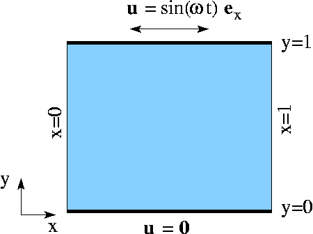

Sketch of the problem.

The flow is governed by the 2D unsteady Navier-Stokes equations,

$Re\left(St\frac{\partial u_i}{\partial t} + u_j\frac{\partial u_i}{\partial x_j}\right) = - \frac{\partial p}{\partial x_i} + \frac{\partial }{\partial x_j} \left( \frac{\partial u_i}{\partial x_j} + \frac{\partial u_j}{\partial x_i} \right) \ \ \ \ \ \ \ \ \ \ (1)$

and the continuity equation

$\frac{\partial u_i}{\partial x_i} = 0 \ \ \ \ \ \ \ \ \ \ (2)$

in the domain

$D = \bigg\{(x_1,x_2) \ | \ x_1 \in [0,1], \ x_2 \in [0,1] \bigg\}.$

We apply the Dirichlet (no-slip) boundary condition

$\left. \mathbf{u}\right|_{\partial D_{lower}}=(0,0), \ \ \ \ \ \ \ \ \ \ (3)$

on the lower, stationary wall, $\partial D_{lower} = \big\{(x_1,x_2) \ | \ x_2=0 \big\}$ , apply the Dirichlet (no-slip) conditions

$\left. \mathbf{u}\right|_{\partial D{upper}}=(\sin\left(\omega t\right),0), \ \ \ \ \ \ \ \ \ \ (4)$

on the upper, moving wall , $\partial D_{upper} = \big\{(x_1,x_2) \ | \ x_2=1 \big\}$ , and apply periodic boundary condition on the "left" and "right" boundaries:

$\left.\mathbf{u}\right|_{x_1=0} = \left.\mathbf{u}\right|_{x_1=1}. \ \ \ \ \ \ \ \ \ \ (5)$

Initial conditions for the velocities are given by

${\bf u}(x_1,x_2,t=0) = {\bf u}_{IC}(x_1,x_2),$

where ${\bf u}_{IC}(x_1,x_2)$ is given.

The exact solution

The above problem has an exact, time-periodic parallel flow solution of the form

${\bf u}_{exact}(x_1,x_2,t) = U(x_2,t) \ {\bf e}_1 \mbox{ \ \ \ \ \ and \ \ \ \ } p_{exact}(x_1,x_2,t) = 0,$

where is governed by

$Re\, St\frac{\partial U}{\partial t} = \frac{\partial^2 U}{\partial x_2^2},$

subject to the boundary conditions and $U(x_2=1,t)=\sin(\omega t)$ . The solution is given by

$U(x_2,t) = Re\left\{\frac{e^{i\omega t}}{e^{i\lambda}-e^{-i\lambda}} \left(e^{i\lambda y}-e^{-i\lambda y}\right)\right\},$

where

$\lambda = i\sqrt{i\omega Re\, St}.$

Results

The two animations below show the computed solutions obtained from a spatial discretisation with Taylor-Hood and Crouzeix-Raviart elements, respectively. In both cases we set $\omega=2\pi, \ Re = ReSt = 10$ and specified the exact, time-periodic solution as the initial condition, i.e. ${\bf u}_{IC}(x_1,x_2) = {\bf u}_{exact}(x_1,x_2,t=0)$ . The computed solutions agree extremely well with the exact solution throughout the simulation.

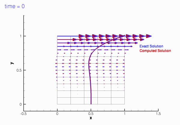
Plot of the velocity field computed with 2D Crouzeix-Raviart elements, starting form the exact, time-periodic solution.

Plot of the velocity field computed with 2D Taylor-Hood elements, starting form the exact, time-periodic solution.

If the simulation is started from other initial conditions, i.e. ${\bf u}_{IC}(x_1,x_2) \ne {\bf u}_{exact}(x_1,x_2,t=0)$ , the velocity field initially differs noticeably from the time-periodic solution ${\bf u}_{exact}(x_1,x_2,t)$ but following the decay of initial transients we have

$\lim_{t\to \infty} {\bf u}(x_1,x_2,t) = {\bf u}_{exact}(x_1,x_2,t).$

This is illustrated in the following plot which shows the evolution of the L2-"error" between the computed and the time-periodic solutions for two different initial conditions. The red line was obtained from a simulation in which ${\bf u}_{IC}(x_1,x_2) = {\bf u}_{exact}(x_1,x_2,t=0)$ ; the blue line was obtained from a computation in which the simulation was started by an "impulsive start", ${\bf u}_{IC}(x_1,x_2) = {\bf 0}$ .

Plot of the L2-'errors' between the computed and time-periodic solution for two different initial conditions.

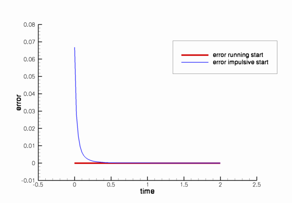
The animations of the simulations for the "impulsive start" (for Taylor-Hood and Crouzeix-Raviart elements) show how the velocity profile approaches the time-periodic solution as the simulation progresses.

The global parameters

As usual, we use a namespace to define the problem parameters, the Reynolds number, , and the Womersley number, $Re\, St$ . We also provide two flags that indicate the length of the run (to allow a short run to be performed when the code is run as a self-test), and the initial condition (allowing a start from ${\bf u}_{exact}$ or an impulsive start in which the fluid is initially at rest).

//===start_of_namespace=================================================
/// Namespace for global parameters
//======================================================================
namespace Global_Parameters
{
 /// Reynolds number
 double Re;
 
 /// Womersley = Reynolds times Strouhal
 double ReSt;
 
 /// Flag for long/short run: Default =  perform long run
 unsigned Long_run_flag=1;
 
 /// Flag for impulsive start: Default = start from exact
 /// time-periodic solution. 
 unsigned Impulsive_start_flag=0;
 
} // end of namespace

The exact solution

We use another namespace to define the exact, time-periodic parallel-flow solution:

//==start_of_exact_solution=============================================
/// Namespace for exact solution
//======================================================================
namespace ExactSoln
{
 
 /// Exact solution of the problem as a vector
 void get_exact_u(const double& t, const Vector<double>& x, Vector<double>& u)
 {
  double y=x[1];
  // I=sqrt(-1)
  complex<double> I(0.0,1.0);
  // omega
  double omega=2.0*MathematicalConstants::Pi;
  // lambda
  complex<double> lambda(0.0,omega*Global_Parameters::ReSt);
  lambda = I*sqrt(lambda);
 
  // Solution
  complex<double> sol(
   exp(complex<double>(0.0,omega*t)) * 
   (exp(lambda*complex<double>(0.0,y))-exp(lambda*complex<double>(0.0,-y)))
   /(exp(I*lambda)-exp(-I*lambda)) );
  
  // Assign real solution
  u.resize(2);
  u[0]=real(sol);
  u[1]=0.0;
 }
 
 /// Exact solution of the problem as a scalar
 void get_exact_u(const double& t, const double& y,double& u)
 {
  // I=sqrt(-1)
  complex<double> I(0.0,1.0);
  // omega
  double omega=2.0*MathematicalConstants::Pi;
  // lambda
  complex<double> lambda(0.0,omega*Global_Parameters::ReSt);
  lambda = I*sqrt(lambda);
  // Solution
  complex<double> sol(
   exp(complex<double>(0.0,omega*t)) * 
   (exp(lambda*complex<double>(0.0,y))-exp(lambda*complex<double>(0.0,-y)))
   /(exp(I*lambda)-exp(-I*lambda)) );
 
  // Assign real solution
  u=real(sol);
 
 }
 
} // end of exact_solution

The driver code

We use optional command line arguments to specify which mode the code is run in: Either as a short or a long run (indicated by the first command line argument being 0 or 1, respectively), and with initial conditions corresponding to an impulsive start or a start from the time-periodic exact solution (indicated by the second command line argument being 1 or 0, respectively). If no command line arguments are specified the code is run in the default mode, specified by the parameter values assigned in the namespace Global_Parameters.

//===start_of_main======================================================
/// Driver code for Rayleigh channel problem
//======================================================================
int main(int argc, char* argv[]) 
{
 
 /// Convert command line arguments (if any) into flags:
 if (argc==1)
  {
   cout << "No command line arguments specified -- using defaults." 
        << std::endl;
  }
 else if (argc==3)
  {
   cout << "Two command line arguments specified:" << std::endl;
   // Flag for long run
   Global_Parameters::Long_run_flag=atoi(argv[1]);
   /// Flag for impulsive start
   Global_Parameters::Impulsive_start_flag=atoi(argv[2]);
  }
 else
  {
   std::string error_message = 
    "Wrong number of command line arguments. Specify none or two.\n";
   error_message +=
    "Arg1: Long_run_flag [0/1]\n";
   error_message +=
    "Arg2: Impulsive_start_flag [0/1]\n";
 
   throw OomphLibError(error_message,
                       OOMPH_CURRENT_FUNCTION,
                       OOMPH_EXCEPTION_LOCATION);
  }
 cout << "Long run flag: " 
      <<  Global_Parameters::Long_run_flag << std::endl;
 cout << "Impulsive start flag: " 
      <<  Global_Parameters::Impulsive_start_flag << std::endl;

Next we set the physical and mesh parameters.

 
 
 // Set physical parameters:
 
 // Womersley number = Reynolds number (St = 1)
 Global_Parameters::ReSt = 10.0;
 Global_Parameters::Re = Global_Parameters::ReSt;
 
 //Horizontal length of domain
 double lx = 1.0;
 
 //Vertical length of domain
 double ly = 1.0;
 
 // Number of elements in x-direction
 unsigned nx=5;
 
 // Number of elements in y-direction
 unsigned ny=10;

Finally we set up DocInfo objects and solve for both Taylor-Hood elements and Crouzeix-Raviart elements.

 
 // Solve with Crouzeix-Raviart elements
 {
  // Set up doc info
  DocInfo doc_info;
  doc_info.number()=0;
  doc_info.set_directory("RESLT_CR");
  
  //Set up problem
  RayleighProblem<QCrouzeixRaviartElement<2>,BDF<2> > problem(nx,ny,lx,ly);
  
  // Run the unsteady simulation
  problem.unsteady_run(doc_info);
 }
 
 
 
 // Solve with Taylor-Hood elements
 {
  // Set up doc info
  DocInfo doc_info;
  doc_info.number()=0;
  doc_info.set_directory("RESLT_TH");
 
  //Set up problem
  RayleighProblem<QTaylorHoodElement<2>,BDF<2> > problem(nx,ny,lx,ly);
  
  // Run the unsteady simulation
  problem.unsteady_run(doc_info);
 }
 
} // end of main

The problem class

The problem class is very similar to that used in the driven cavity example. We specify the type of the element and the type of the timestepper (assumed to be a member of the BDF family) as template parameters and pass the mesh parameters to the problem constructor.

//===start_of_problem_class=============================================
/// Rayleigh-type problem: 2D channel whose upper
/// wall oscillates periodically.
//======================================================================
template<class ELEMENT, class TIMESTEPPER>
class RayleighProblem : public Problem
{
public:
 
 /// Constructor: Pass number of elements in x and y directions and 
 /// lengths
 RayleighProblem(const unsigned &nx, const unsigned &ny, 
                 const double &lx, const double &ly);

No action is needed before or after solving, but we update the time-dependent boundary conditions at the upper wall before each timestep, using Problem::actions_before_implicit_timestep(). The boundary values are obtained from the exact solution, defined in the namespace ExactSoln.

 
 //Update before solve is empty
 void actions_before_newton_solve() {}
 
 /// Update after solve is empty
 void actions_after_newton_solve() {}
 
 //Actions before timestep: Update no slip on upper oscillating wall
 void actions_before_implicit_timestep()
  {
   // No slip on upper boundary
   unsigned ibound=2;
   unsigned num_nod=mesh_pt()->nboundary_node(ibound);
   for (unsigned inod=0;inod<num_nod;inod++)
    {
     // Get exact solution
     double y=mesh_pt()->boundary_node_pt(ibound,inod)->x(1);
     double time=time_pt()->time();
     double soln;
     ExactSoln::get_exact_u(time,y,soln);
     
     // Assign exact solution to boundary
     mesh_pt()->boundary_node_pt(ibound,inod)->set_value(0,soln);
     mesh_pt()->boundary_node_pt(ibound,inod)->set_value(1,0.0);
    }
 
  } // end of actions_before_implicit_timestep

The function unsteady_run(...), discussed below, performs the timestepping and documents the solution in the directory specified in the DocInfo object.

   
 /// Run an unsteady simulation
 void unsteady_run(DocInfo& doc_info); 

We define the function doc_solution(...) which documents the results, and provide functions to set the initial conditions and to fix a pressure value. The problem's only member data contains an output stream in which we record the time-trace of the solution.

 
 /// Doc the solution
 void doc_solution(DocInfo& doc_info);
 
 /// Set initial condition (incl previous timesteps) according
 /// to specified function. 
 void set_initial_condition();
 
private:
 
 /// Fix pressure in element e at pressure dof pdof and set to pvalue
 void fix_pressure(const unsigned &e, const unsigned &pdof, 
                   const double &pvalue)
  {
   //Cast to proper element and fix pressure
   dynamic_cast<ELEMENT*>(mesh_pt()->element_pt(e))->
                          fix_pressure(pdof,pvalue);
  }
 
 /// Trace file
 ofstream Trace_file;
 
}; // end of problem_class

The problem constructor

We start by building the timestepper, determining its type from the class's second template argument, and pass a pointer to it to the Problem, using the function Problem::add_time_stepper_pt(...).

//===start_of_constructor=============================================
/// Problem constructor
//====================================================================
template<class ELEMENT,class TIMESTEPPER>
RayleighProblem<ELEMENT,TIMESTEPPER>::RayleighProblem
(const unsigned &nx, const unsigned &ny,
 const double &lx, const double& ly)
{
 //Allocate the timestepper
 add_time_stepper_pt(new TIMESTEPPER); 

Next we build the mesh and pass an additional boolean flag to the constructor to indicate that periodic boundary conditions are to be applied in the -direction. We will discuss the implementation of this feature in more detail in below.

 
 //Now create the mesh with periodic boundary conditions in x direction
 bool periodic_in_x=true;
 Problem::mesh_pt() = 
  new RectangularQuadMesh<ELEMENT>(nx,ny,lx,ly,periodic_in_x,
                                   time_stepper_pt());

We pin both velocity components on the top and bottom boundaries (i.e. at and , respectively), and pin the vertical velocity on the left and right boundaries (i.e. at and , respectively) to enforce horizontal outflow through the periodic boundaries.

 
 // Set the boundary conditions for this problem: All nodes are
 // free by default -- just pin the ones that have Dirichlet conditions
 // here
 unsigned num_bound=mesh_pt()->nboundary();
 for(unsigned ibound=0;ibound<num_bound;ibound++)
  {
   unsigned num_nod=mesh_pt()->nboundary_node(ibound);
   for (unsigned inod=0;inod<num_nod;inod++)
    {
     // No slip on top and bottom
     if ((ibound==0)||(ibound==2))
      {
       mesh_pt()->boundary_node_pt(ibound,inod)->pin(0);
       mesh_pt()->boundary_node_pt(ibound,inod)->pin(1);
      }
     // Horizontal outflow on the left (and right -- right bc not
     // strictly necessary because of symmetry)
     else if ((ibound==1)||(ibound==3))
      {
       mesh_pt()->boundary_node_pt(ibound,inod)->pin(1);
      }
    }
  } // end loop over boundaries

Finally we pass the pointers to the Reynolds and Strouhal numbers, and $Re\, St$ , to the elements. Since no traction boundary conditions are applied anywhere, the pressure is only determined up to an arbitrary constant. To ensure a unique solution we pin a single pressure value before setting up the equation numbering scheme.

 
 //Complete the problem setup to make the elements fully functional
 
 //Loop over the elements
 unsigned n_el = mesh_pt()->nelement();
 for(unsigned e=0;e<n_el;e++)
  {
   //Cast to a fluid element
   ELEMENT *el_pt = dynamic_cast<ELEMENT*>(mesh_pt()->element_pt(e));
 
   //Set the Reynolds number, etc
   el_pt->re_pt() = &Global_Parameters::Re;
   el_pt->re_st_pt() = &Global_Parameters::ReSt;
  }
 
 // Now pin the pressure in first element at value 0 to 0.0
 fix_pressure(0,0,0.0);
 
 //Assgn equation numbers
 cout << assign_eqn_numbers() << std::endl; 
} // end of constructor

Initial conditions

The application of initial conditions for vector-valued problems is performed by the same procedure that we described for scalar problems, except that we now have to assign "history values" for multiple nodal values. For timesteppers from the BDF family, the "history values" represent the solution at previous timesteps. We check that the timestepper is of the appropriate type,
loop over previous time levels, determine the velocity at those times and assign them to the "history values" of the velocities. No initial conditions are required for the pressure. Note that we also have to assign "history values" for the nodal positions since oomph-lib's Navier-Stokes elements discretise the momentum equations in their ALE form. This aspect was explained in more detail in our discussion of the solution of the unsteady heat equation.

//======================start_of_set_initial_condition====================
/// Set initial condition: Assign previous and current values
/// from exact solution.
//========================================================================
template<class ELEMENT,class TIMESTEPPER>
void RayleighProblem<ELEMENT,TIMESTEPPER>::set_initial_condition()
{ 
 
 // Check that timestepper is from the BDF family
 if (time_stepper_pt()->type()!="BDF")
  {
   std::ostringstream error_stream;
   error_stream << "Timestepper has to be from the BDF family!\n"
                << "You have specified a timestepper from the "
                << time_stepper_pt()->type() << " family" << std::endl;
 
   throw OomphLibError(error_stream.str(),
                       OOMPH_CURRENT_FUNCTION,
                       OOMPH_EXCEPTION_LOCATION);
  }
 
 // Backup time in global Time object
 double backed_up_time=time_pt()->time();
         
 // Past history needs to be established for t=time0-deltat, ...
 // Then provide current values (at t=time0) which will also form
 // the initial guess for the first solve at t=time0+deltat
 
 // Vector of exact solution value
 Vector<double> soln(2);
 Vector<double> x(2);
 
 //Find number of nodes in mesh
 unsigned num_nod = mesh_pt()->nnode();
 
 // Set continuous times at previous timesteps:
 // How many previous timesteps does the timestepper use?
 int nprev_steps=time_stepper_pt()->nprev_values();
 Vector<double> prev_time(nprev_steps+1);
 for (int t=nprev_steps;t>=0;t--)
  {
   prev_time[t]=time_pt()->time(unsigned(t));
  } 
 
 // Loop over current & previous timesteps
 for (int t=nprev_steps;t>=0;t--)
  {
   // Continuous time
   double time=prev_time[t];
   cout << "setting IC at time =" << time << std::endl;
   
   // Loop over the nodes to set initial guess everywhere
   for (unsigned n=0;n<num_nod;n++)
    {
     // Get nodal coordinates
     x[0]=mesh_pt()->node_pt(n)->x(0);
     x[1]=mesh_pt()->node_pt(n)->x(1);
 
     // Get exact solution at previous time
     ExactSoln::get_exact_u(time,x,soln);
     
     // Assign solution
     mesh_pt()->node_pt(n)->set_value(t,0,soln[0]);
     mesh_pt()->node_pt(n)->set_value(t,1,soln[1]);
     
     // Loop over coordinate directions: Mesh doesn't move, so 
     // previous position = present position
     for (unsigned i=0;i<2;i++)
      {
       mesh_pt()->node_pt(n)->x(t,i)=x[i];
      }
    } 
  }
 
 // Reset backed up time for global timestepper
 time_pt()->time()=backed_up_time;
 
} // end of set_initial_condition

Post processing

The function doc_solution(...) is similar to those used in the unsteady heat examples. We plot the computed solution, the time-periodic exact solution and the difference between the two, and record various parameters in the trace file. The plot of the computed solution contains tecplot instructions that generate a blue line in the top-left corner of the plot to indicate how time progresses during the simulation. The trace file contains a record of

the value of the continuous time, ,
the coordinates of a control node, $(x_1^{[c]},x_2^{[c]})$ ,
the computed velocity at the control node, $( u_1^{[c]},u_2^{[c]})$ ,
the time-periodic solution, evaluated at the control node, $(u_1^{[c,exact]},u_2^{[c,exact]})$ ,
the difference between the computed velocities and the time-periodic solution at the control node,
the L2 norm of the "error" between the computed and time-periodic solution for the velocity, and
the L2 norm of the time-periodic solution for the velocity.

//==start_of_doc_solution=================================================
/// Doc the solution
//========================================================================
template<class ELEMENT,class TIMESTEPPER>
void RayleighProblem<ELEMENT,TIMESTEPPER>::doc_solution(DocInfo& doc_info)
{ 
 ofstream some_file;
 char filename[100];
 
 // Number of plot points
 unsigned npts=5; 
 
 // Output solution 
 sprintf(filename,"%s/soln%i.dat",doc_info.directory().c_str(),
         doc_info.number());
 some_file.open(filename);
 mesh_pt()->output(some_file,npts);
 
 // Write file as a tecplot text object
 some_file << "TEXT X=2.5,Y=93.6,F=HELV,HU=POINT,C=BLUE,H=26,T=\"time = " 
           << time_pt()->time() << "\"";
 // ...and draw a horizontal line whose length is proportional
 // to the elapsed time
 some_file << "GEOMETRY X=2.5,Y=98,T=LINE,C=BLUE,LT=0.4" << std::endl;
 some_file << "1" << std::endl;
 some_file << "2" << std::endl;
 some_file << " 0 0" << std::endl;
 some_file << time_pt()->time()*20.0 << " 0" << std::endl;
 
 some_file.close();
 
 // Output exact solution 
 //----------------------
 sprintf(filename,"%s/exact_soln%i.dat",doc_info.directory().c_str(),
         doc_info.number());
 some_file.open(filename);
 mesh_pt()->output_fct(some_file,npts,time_pt()->time(),
                       ExactSoln::get_exact_u); 
 some_file.close();
 
 // Doc error
 //----------
 double error,norm;
 sprintf(filename,"%s/error%i.dat",doc_info.directory().c_str(),
         doc_info.number());
 some_file.open(filename);
 mesh_pt()->compute_error(some_file,
                          ExactSoln::get_exact_u,
                          time_pt()->time(),
                          error,norm); 
 some_file.close();
 
 // Doc solution and error
 //-----------------------
 cout << "error: " << error << std::endl; 
 cout << "norm : " << norm << std::endl << std::endl;
 
 // Get time, position and exact soln at control node 
 unsigned n_control=37;
 Vector<double> x(2), u(2);
 double time=time_pt()->time();
 Node* node_pt=
  dynamic_cast<ELEMENT*>(mesh_pt()->element_pt(n_control))->node_pt(1);
 x[0] = node_pt->x(0);
 x[1] = node_pt->x(1);
 ExactSoln::get_exact_u(time,x,u);
 
 // Write trace file
 Trace_file << time << " " 
            << x[0] << " "
            << x[1] << " "
            << node_pt->value(0) << " "
            << node_pt->value(1) << " "
            << u[0] << " "
            << u[1] << " " 
            << abs(u[0]-node_pt->value(0)) << " "
            << abs(u[1]-node_pt->value(1)) << " " 
            << error << " "
            << norm << " "
            << std::endl;
 
 
} // end_of_doc_solution   

The timestepping loop

The function unsteady_run(...) is used to perform the timestepping procedure. We start by opening the trace file and write a suitable header for the visualisation with tecplot.

//===start_of_unsteady_run=====================================================
/// Unsteady run...
//=============================================================================
template<class ELEMENT,class TIMESTEPPER>
void RayleighProblem<ELEMENT,TIMESTEPPER>::unsteady_run(DocInfo& doc_info)
{
 
 // Open trace file
 char filename[100];   
 sprintf(filename,"%s/trace.dat",doc_info.directory().c_str());
 Trace_file.open(filename);
 
 // Write tecplot header for trace file
 Trace_file << "time" << ",      " 
            << "x" << ",         "
            << "y" << ",         "
            << "u_1" << ",       "
            << "u_2" << ",       "
            << "u_exact_1" << ", "
            << "u_exact_2" << ", "
            << "error_1" << ",   "
            << "error_2" << ",   " 
            << "L2 error" << ",  "
            << "L2 norm" << ",   " << std::endl;

Next, we choose a value for the timestep and set up the initial conditions, either for an impulsive start...

 
 //Set value of dt
 double dt = 0.025;
 
 if (Global_Parameters::Impulsive_start_flag==1)
  {
   // Initialise all history values for an impulsive start
   assign_initial_values_impulsive(dt);
   cout << "IC = impulsive start" << std::endl;
  }

...or for a "smooth" start from the time-periodic exact solution:

 else
  {
   // Initialise timestep
   initialise_dt(dt);
   // Set initial conditions.
   set_initial_condition();
   cout << "IC = exact solution" << std::endl;
  } 

We choose the number of timesteps to be computed and document the initial conditions.

 
 //Now do many timesteps
 unsigned ntsteps=80;
 
 // If validation run only do 5 timesteps
 if (Global_Parameters::Long_run_flag==0)
  { 
   ntsteps=5; 
   cout << "validation run" << std::endl;
  }
 
 // Doc initial condition
 doc_solution(doc_info);
 
 // increment counter
 doc_info.number()++;

Finally, perform the actual timestepping and document the solution after every timestep.

 
 //Loop over the timesteps
 for(unsigned t=1;t<=ntsteps;t++)
  {
   cout << "TIMESTEP " << t << std::endl;
   
   //Take one fixed timestep
   unsteady_newton_solve(dt);
 
   //Output the time
   cout << "Time is now " << time_pt()->time() << std::endl;
 
   // Doc solution
   doc_solution(doc_info);
 
   // increment counter
   doc_info.number()++;
  }
 
} // end of unsteady run

Comments and Exercises

Periodic boundaries

A key feature of the current problem is the presence of periodic boundary conditions. The application of the periodic boundary condition is performed "inside" the mesh constructor and details of the implementation were therefore "hidden". We will now discuss the steps required to apply periodic boundary conditions and explain why it is easier to apply periodic boundary conditions in the mesh constructor rather than in the "driver code".

Periodic boundary conditions arise in problems that are periodic in one of their coordinate directions. It is important to realise that, even though the solution at the corresponding nodes on the two periodic domain boundaries (the left and the right boundary in the above example) are the same, one of their nodal coordinates differs. For instance, in the above example, each of the nodes on the left boundary has the same velocity values and the same -coordinate as its corresponding (periodic) node on the right boundary. However, the -coordinate of the nodes on the left boundary is , whereas that of the (periodic) nodes on the right boundary is . It is therefore not possible to regard the nodes as identical.

In oomph-lib we create periodic nodes by allowing two (or more) nodes to access some of the same internal data. One of the nodes should be regarded as the original and the other(s) are set to be its "periodic counterpart(s)" and hence access its internal data. The "periodic counterpart(s)" are created by calling the member function

BoundaryNode::make_periodic(Node *const& node_pt)

where the pointer to the original node is passed as the argument. Note that the required functionality imposes a slight storage overhead and so in oomph-lib we only allow BoundaryNodes to be made periodic.

Here is a sketch of a 2D rectangular quad mesh. If this mesh is to be used in a problem with periodic boundary conditions in the horizontal direction (as in the above example), the pointer to node 3 on boundary 3 would have to be used when node 3 on boundary 1 is made periodic, etc. The appropriate commands are

//Get pointers to the two nodes that are to be "connected" via
//a periodic boundary
Node* original_node_pt = mesh_pt()->boundary_node_pt(3,3);
Node* periodic_node_pt = mesh_pt()->boundary_node_pt(1,3);
 
//Make the periodic_node_pt periodic the data from the original_node_pt
periodic_node_pt->make_periodic(original_node_pt);

Figure of a mesh that is periodic in the horizontal direction.

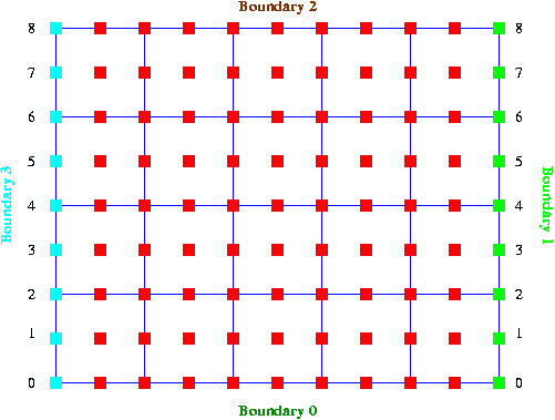
Although it is possible to make nodes periodic at any time, it is usually easier to determine which nodes should be "connected" during mesh construction. We therefore strongly recommend to implement periodic boundary conditions inside the mesh constructor. The source code for the constructor of the

RectangularQuadMesh<ELEMENT>

that we used in the above problem, illustrates a possible implementation.

Periodic boundaries in spatially adaptive computations

We note that the application of periodic boundary conditions in spatially adaptive computations is slightly more complicated because of the possible presence of hanging nodes on the periodic boundaries. We refer to another tutorial for a discussion of this aspect.

Exercises

Show that in the present problem the time-periodic solution can also be obtained without applying periodic boundary conditions. Show this mathematically and "by trial and error" (i.e. by changing the boolean flag that is passed to the mesh constructor). Explain why the number of unknowns increases when no periodic boundary conditions are applied.
Confirm that the assignment of "history values" for the nodal positions in set_initial_conditions() is essential.

Source files for this tutorial

The source files for this tutorial are located in the directory: demo_drivers/navier_stokes/rayleigh_channel/
The driver code is: demo_drivers/navier_stokes/rayleigh_channel/rayleigh_channel.cc

PDF file

A pdf version of this document is available.