We study the problem of the motion of a rigid elliptical particle freely suspended in a shear flow as described by Jeffery (1922) [The motion of elliptical particles immersed in viscous fluid, Proc. Roy. Soc. A 102 161-179]. The problem is solved using oomph-lib's inline unstructured mesh generation procedures to modify the fluid mesh in response to changes in orientation of the ellipse.

Overview of the problem

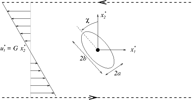
A rigid ellipse immersed in a shear flow

We consider an ellipse with centre of mass fixed at the origin of a Cartesian coordinate system $(x_{1}^{*}, x_{2}^{*})$ , but immersed in a viscous fluid undergoing a linear shear flow with shear rate . In the absence of the ellipse the fluid velocity field would be $u^{*}_{1} = Gx^{*}_{2}$ , $u^{*}_{2} = 0$ , where $u^{*}_{i}$ is the dimensional velocity component in the $x^{*}_{i}$ coordinate direction.

The configuration of a rigid body in two dimensions is determined entirely by the position of its centre of mass, $(X^{*}_{1},X^{*}_{2})$ and an angle, $\chi$ that specifies its orientation to a fixed axis. The equations governing the motion of the particle are then simply conservation of linear and angular momentum:

$M \frac{\mbox{d}^{2} X^{*}_{i}}{\mbox{d} t^{*2}} = F^{*}_{i} \quad \mbox{and} \quad I \frac{\mbox{d}^{2} \chi}{\mbox{d} t^{*2}} = T^{*},$

where is the mass of the body, is its moment of inertia about the centre of mass, $(F^{*}_{1},F^{*}_{2})$ is the resultant force on the body and $T^{*}$ is the resultant torque about the centre of mass.

In the present context, the force and torque on the body are entirely due to the viscous fluid loading on its surface in which case

$F^{*}_{i} = \int \tau^{*}_{ij}\, n_{j}\, \mbox{d} s \quad\mbox{and}\quad T^{*} = \oint (x^{*}_{1} - X^{*}_{1}) \tau^{*}_{2j}\,n_{j} - (x^{*}_{2} - X^{*}_{2}) \tau^{*}_{1j}\,n_{j}\, \mbox{d} s,$

where the integral is around the perimeter of the ellipse, $\tau^{*}_{ij}$ is the fluid stress tensor and $(n_{1},n_{2})$ is the unit normal to the ellipse surface, directed away from the solid body.

We non-dimensionalise the rigid-body equations, using the same problem-specific reference quantities as used in the non-dimensionalisation of the Navier–Stokes equations, described in another tutorial. Thus, ${\cal U}$ is a typical fluid velocity, ${\cal L}$ is the length scale, ${\cal T}$ is the time scale and the fluid pressure is non-dimensionalised on the viscous scale, $\mu_{ref} {\cal U}/{\cal L}$ , where $\mu_{ref}$ is the reference fluid viscosity. Hence,

$\tau^{*}_{ij} = \frac{\mu_{ref} {\cal U}}{{\cal L}} \, \tau_{ij}, \qquad x_i^{*} = {\cal L}\, x_i, \qquad X_i^* = {\cal L}\, X_i, \qquad t^* = {\cal T}\, t.$

The external forces and torques are non-dimensionalised on the viscous scales per unit length, $F^{*}_{i} = \mu_{ref} {\cal U} F_{i}$ and $T^{*} = \mu_{ref} {\cal U} {\cal L} T$ . The dimensionless rigid-body equations are then

$Re St^{2} \frac{\rho_{s}}{\rho_{f}}\, \bar{M}\, \frac{\mbox{d}^{2} X_{i}}{\mbox{d} t^{2}} = F_{i} \quad \mbox{and} \quad Re St^{2} \frac{\rho_{s}}{\rho_{f}}\, \bar{I}\, \frac{\mbox{d}^{2} \chi}{\mbox{d} t^{2}} = T,$

where the dimensionless parameters

$Re = \frac{\rho_{f} {\cal U}{\cal L}}{\mu_{ref}}, \quad St = \frac{\cal L}{{\cal U}{\cal T}},\quad \frac{\rho_{s}}{\rho_{f}}, \quad \bar{M} = \frac{M}{\rho_{s} {\cal L}^{2}}, \quad \bar{I} = \frac{I}{\rho_{s} {\cal L}^{4}},$

are the Reynolds number, the Strouhal number, the density ratio, and the dimensionless mass and moment of inertia, respectively. In the above $\rho_{f}$ is the fluid density and $\rho_{s}$ is the solid density.

In the specific problem considered here, the centre of mass is fixed, and the only possible motion of the particle is free rotation. The particle motion is therefore reduced to the solution of a single equation for the unknown angle. We choose ${\cal L} = 2b$ , the major axis of the ellipse, ${\cal U} = 2Gb$ and ${\cal T} = G^{-1}$ , so that and the governing equations for the fluid and solid become

$Re \left (\frac{\partial u_i}{\partial t} + u_j \frac{\partial u_i}{\partial x_j} \right) = - \frac{\partial p}{\partial x_i} + \frac{\partial }{\partial x_j} \left[ \frac{\partial u_i}{\partial x_j} + \frac{\partial u_j}{\partial x_i} \right] \quad\mbox{and}\quad \frac{\partial u_i}{\partial x_i} = 0.$

and

$Re \left(\frac{\rho_{s}}{\rho_{f}}\right) \bar{I} = \oint \left[x_{1}\tau_{2j}\,n_{j} - x_{2} \tau_{1j}\,n_{j}\, \right] \mbox{d} s,$

We perform the computations in the domain $x_{1} \in [-L, L]$ and $x_{2} \in [-H, H]$ , and apply the boundary conditions

$u_{1} = H f(t), u_{2} = 0, \quad\mbox{on}\quad x_{2} = -H;$

$u_{1} = -H f(t), u_{2} = 0, \quad\mbox{on}\quad x_{2} = H;$

$\tau_{11} = 0, u_{2} = 0, \quad\mbox{on}\quad x_{1} = -L, L;$

where

is a smooth ramp function such that $f(0) = \dot{f}(0) = \ddot{f}(0) = 0$ and $f(t) \to 1$ as $t \to \infty$ .

Results

Jeffery (1922) showed that for a two-dimensional ellipse in Stokes flow ( ), the exact solution for the angle as a function of time is

$\chi = \tan^{-1}\left(\frac{b}{a}\tan \frac{abGt}{a^{2} + b^{2}}\right),\quad\mbox{and}\quad \dot{\chi} = \frac{G}{a^{2} + b^{2}}\left(b^{2}\cos^{2}\chi + a^{2}\sin^{2}\chi\right).$

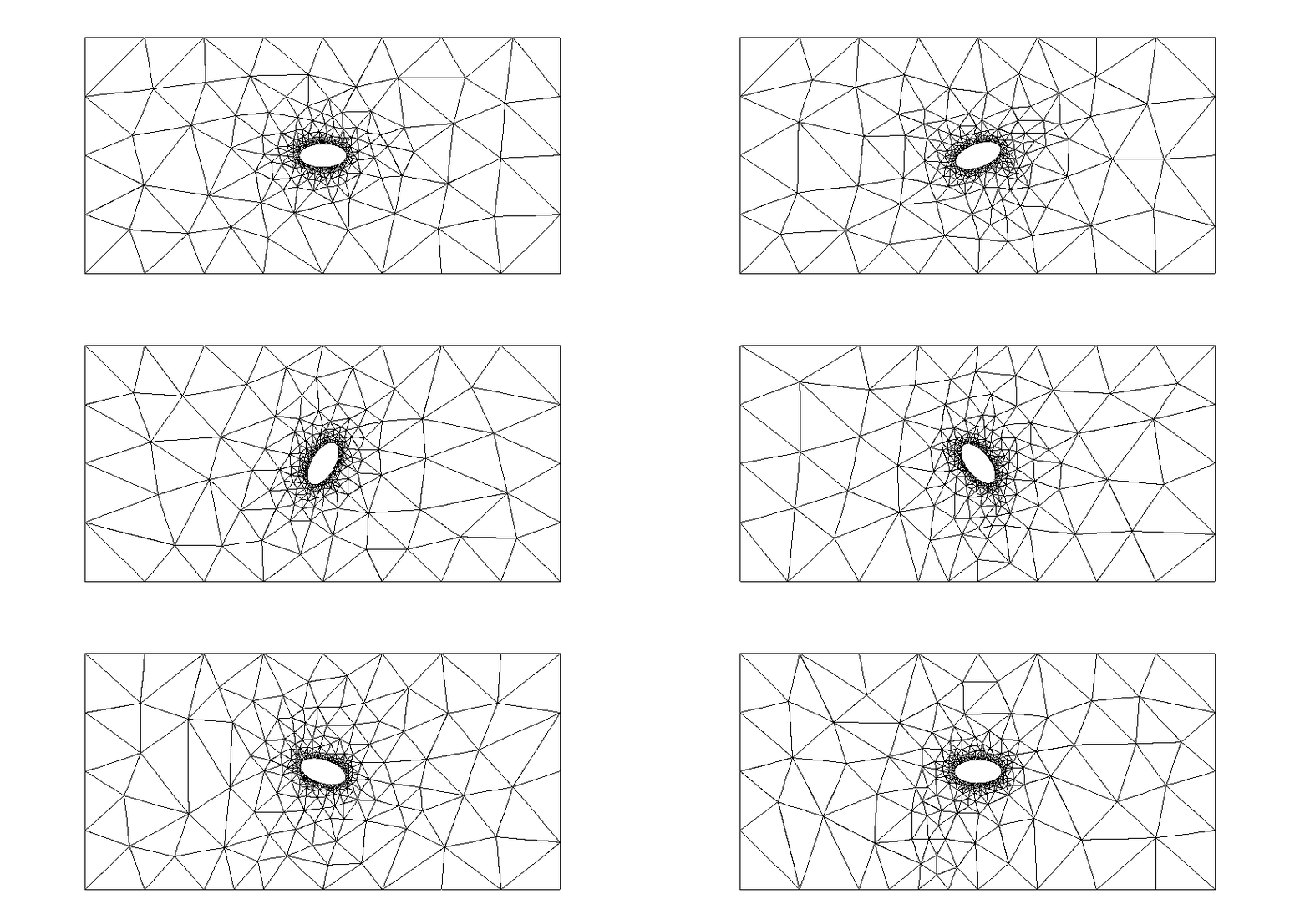
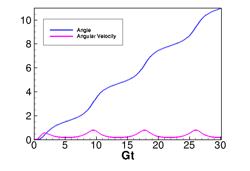
Thus, the ellipse performs periodic orbits but with a non-uniform velocity. For sufficiently small , Ding & Aidun (2000) [The dynamics and scaling law for particles suspended in shear flow with inertia, J. Fluid Mech. 423 317-344] showed that the system approximates the Jeffery orbits but with an increased period. Typical solutions for are shown below.

An ellipse performing approximate Jeffery orbits at Re = 1

Angle and angular velocity as functions of time for Re = 1

Implementation as a fluid-structure interaction problem

The problem is a fluid-structure interaction problem in which the structural dynamics are particularly simple, depending only on a single degree of freedom. Nonetheless, the two types of physical coupling between the fluid and the solid remain:

The position of the free boundary depends on the position of the rigid body.
The rigid body is loaded by the fluid traction.

As in other 2D unstructured FSI problems, we treat the fluid mesh as a pseudo-solid body and determine the position of the boundary nodes on the fluid-solid interface using
ImposeDisplacementByLagrangeMultiplierElements.

The rigid body mechanics is handled by using a GeomObject that represents the perimeter of the rigid body to create an ImmersedRigidBodyElement that solves the three equations of motion for a rigid body; and the load is applied to the rigid body using NavierStokesSurfaceDragTorqueElements.

Problem Parameters

We use a namespace to define the parameters used in the problem

//==start_of_namespace==============================
/// Namespace for Problem Parameters
//==================================================
 namespace Problem_Parameter
 {    
  /// Reynolds number
  double Re=1.0;
 
  /// Strouhal number
  double St = 1.0;
 
  /// Density ratio (Solid density / Fluid density)
  double Density_ratio = 1.0;
 
  /// Initial axis of the elliptical solid in x-direction
  double A = 0.25;
  
  /// Initial axis of the elliptical solid in y-direction
  /// (N.B. 2B = 1 is the reference length scale)
  double B = 0.5;
 
  /// Pseudo-solid (mesh) Poisson ratio
  double Nu=0.3;
 
  /// Pseudo-solid (mesh) "density" 
  /// Set to zero because we don't want inertia in the node update!
  double Lambda_sq=0.0;
 
  /// Constitutive law used to determine the mesh deformation
  ConstitutiveLaw *Constitutive_law_pt=   
   new GeneralisedHookean(&Problem_Parameter::Nu);
 
 } // end_of_namespace

Defining the ellipse as a GeomObject

We create a basic GeomObject to represent the ellipse whose boundary we parametrise by the polar angle, measured from its centre of mass.

//===================start_of_general_ellipse=================================
/// A geometric object for an ellipse with initial centre of mass at
/// (centre_x, centre_y) with axis in the x direction given by 2a
/// and in the y-direction given by 2b. The boundary of the ellipse is
/// parametrised by its angle.
//============================================================================
class GeneralEllipse : public GeomObject
{
private:
 
 //Storage for the centre of mass and semi-major and semi-minor axes
 double Centre_x, Centre_y, A, B;
 
public:
 
 /// Simple Constructor that transfers appropriate geometric 
 /// parameters into internal data
 GeneralEllipse(const double &centre_x, const double &centre_y,
                const double &a, const double &b)
  : GeomObject(1,2), Centre_x(centre_x), Centre_y(centre_y), A(a), B(b)
  {}
 
 /// Empty Destructor
 ~GeneralEllipse() {}
 
 /// Return the position of the ellipse boundary as a function of 
 /// the angle xi[0]
 void position(const Vector<double> &xi, Vector<double> &r) const
  {
   r[0] = Centre_x + A*cos(xi[0]);
   r[1] = Centre_y + B*sin(xi[0]);
  }
 
 //Return the position which is always fixed
 void position(const unsigned &t,
               const Vector<double> &xi, Vector<double> &r) const
  {
   return position(xi,r);
  }
 
};
//end_of_general_ellipse

The driver code

After parsing the command-line arguments, which are used to modify certain parameters for validation runs, a single instance of the UnstructuredImmersedEllipseProblem (described below) is constructed using Taylor Hood elements.

//==========start_of_main======================================
/// Driver code for immersed ellipse problem
//============================================================
int main(int argc, char **argv)
{
 // Store command line arguments
 CommandLineArgs::setup(argc,argv);
 
 // Define possible command line arguments and parse the ones that
 // were actually specified
 
 // Validation?
 CommandLineArgs::specify_command_line_flag("--validation");
 
 // Parse command line
 CommandLineArgs::parse_and_assign(); 
 
 // Doc what has actually been specified on the command line
 CommandLineArgs::doc_specified_flags();
  
 // Create problem in initial configuration
 UnstructuredImmersedEllipseProblem<
 ProjectableTaylorHoodElement<MyTaylorHoodElement> > problem;  

After construction the Nodes on the boundary of the ellipse will have been directly mapped onto the curvilinear surface using a strong (collocation) condition, $x_{i} = R_{i}$ , where $R_{i}$ is the corresponding boundary of the ellipse. In the full problem the displacement boundary condition is enforced weakly via Lagrange multipliers $\oint \left\{x_{i} - R_{i}\right\}\psi \mbox{d} s = 0$ . In order to ensure consistency, we initially solve the problem in which the rigid body is pinned so that the boundary nodes are adjusted to be consistent with the weak form of the boundary condition. We note that for sufficiently fine initial meshes the difference is minimal.

 
 //Initially ensure that the nodal positions are consistent with 
 //their weak imposition
 problem.solve_for_consistent_nodal_positions();

Now that we have a consistent initial condition, we initialise the timestepper and set conditions consistent with a impulsive start from rest.

 
 // Initialise timestepper
 double dt=0.05;
 problem.initialise_dt(dt);
 
 // Perform impulsive start
 problem.assign_initial_values_impulsive();
 
 // Output initial conditions
 problem.doc_solution();

We then take a fixed number of timesteps on the initial mesh, documenting the solution after each solve.

 
 // Solve problem a few times on given mesh
 unsigned nstep=3;
 for (unsigned i=0;i<nstep;i++)
  {
   // Solve the problem
   problem.unsteady_newton_solve(dt);    
   problem.doc_solution();
  }

Finally, we loop over a number of `‘cycles’' in which we adapt the problem and then solve for a fixed number of time steps on the each mesh.

 for (unsigned j=0;j<ncycle;j++)
  {       
   // Adapt the problem
   problem.adapt();
 
   //Solve problem a few times
   for (unsigned i=0;i<nstep;i++)
    {     
     // Solve the problem
     problem.unsteady_newton_solve(dt);
     problem.doc_solution();
    }
  }
 
} //end of main

The Problem class

The Problem class follows the usual pattern. The time-dependent boundary conditions are applied using the actions_before_implicit_timestep() function and the no-slip boundary condition is applied in actions_before_newton_convergence_check() via an auxiliary node update function.

Recall that when adapting an unstructured mesh, its constituent elements are completely re-generated. Physical parameters and boundary conditions must therefore be reassigned, which is the task of the complete_problem_setup() function, called in actions_after_adapt(). Helper functions are also provided to solve the initial problem to move the boundary nodes [solve_for_consistent_nodal_positions()]; to apply the boundary conditions [set_boundary_velocity()]; and to construct and delete the surface elements that impose the Lagrange multiplier constraints and compute the load on the rigid body [create_lagrange_multiplier_elements(), delete_lagrange_multiplier_elements(), create_drag_elements(), delete_drag_elements()].

The class also provides storage for the meshes, the rigid body and file handles for documentation.

//==start_of_problem_class============================================
/// Unstructured Navier-Stokes ALE Problem for a rigid ellipse 
/// immersed within a viscous fluid
//====================================================================
template<class ELEMENT>
class UnstructuredImmersedEllipseProblem : public Problem
{
 
public:
 
 /// Constructor
 UnstructuredImmersedEllipseProblem();
 
 /// Destructor
 ~UnstructuredImmersedEllipseProblem();
 
 /// Reset the boundary conditions when timestepping
 void actions_before_implicit_timestep()
  {
   this->set_boundary_velocity();
  }
 
 /// Wipe the meshes of Lagrange multiplier and drag elements
 void actions_before_adapt();
 
 /// Rebuild the meshes of Lagrange multiplier and drag elements
 void actions_after_adapt();
 
 /// Re-apply the no slip condition (imposed indirectly via dependent
 /// velocities)
 void actions_before_newton_convergence_check()
  {
   // Update mesh -- this applies the auxiliary node update function
   Fluid_mesh_pt->node_update();
  }
 
 /// Set boundary condition, assign auxiliary node update fct.
 /// Complete the build of all elements, attach power elements that allow
 /// computation of drag vector
 void complete_problem_setup();
 
 /// Set the boundary velocity
 void set_boundary_velocity();
 
 /// Function that solves a simplified problem to ensure that 
 /// the positions of the boundary nodes are initially consistent with
 /// the lagrange multiplier formulation
 void solve_for_consistent_nodal_positions();
 
 /// Doc the solution
 void doc_solution(const bool& project=false);
  
 /// Output the exact solution
 void output_exact_solution(std::ofstream &output_file);
 
private:
 
 /// Create elements that enforce prescribed boundary motion
 /// for the pseudo-solid fluid mesh by Lagrange multipliers
 void create_lagrange_multiplier_elements();
 
 /// Delete elements that impose the prescribed boundary displacement
 /// and wipe the associated mesh
 void delete_lagrange_multiplier_elements();
 
 /// Create elements that calculate the drag and torque on
 /// the boundaries
 void create_drag_elements();
 
 /// Delete elements that calculate the drag and torque on the 
 /// boundaries
 void delete_drag_elements();
 
 /// Pin the degrees of freedom associated with the solid bodies
 void pin_rigid_body();
 
 /// Unpin the degrees of freedom associated with the solid bodies
 void unpin_rigid_body();
 
 /// Pointers to mesh of Lagrange multiplier elements
 SolidMesh* Lagrange_multiplier_mesh_pt;
 
 /// Pointer to Fluid_mesh
 RefineableSolidTriangleMesh<ELEMENT>* Fluid_mesh_pt;
 
 /// Triangle mesh polygon for outer boundary 
 TriangleMeshPolygon* Outer_boundary_polygon_pt;
 
 /// Mesh of drag elements
 Vector<Mesh*> Drag_mesh_pt;
 
 /// Mesh of the generalised elements for the rigid bodies
 Mesh* Rigid_body_mesh_pt;
 
 /// Storage for the geom object
 Vector<GeomObject*> Rigid_body_pt;
 
 /// Internal DocInfo object
 DocInfo Doc_info;
 
 /// File to document the norm of the solution (for validation purposes)
 ofstream Norm_file;
 
 /// File to document the motion of the centre of gravity
 ofstream Cog_file;
 
 /// File to document the exact motion of the centre of gravity
 ofstream Cog_exact_file;
 
}; // end_of_problem_class

The Problem Constructor

We begin by opening the output files and allocating two time steppers, one for the fluid problem and one for the rigid body problem.

//==start_constructor=====================================================
/// Constructor: Open output files, construct time steppers, build 
///  fluid mesh, immersed rigid body and combine to form the problem
//========================================================================
template<class ELEMENT>
UnstructuredImmersedEllipseProblem<ELEMENT>::
UnstructuredImmersedEllipseProblem()
{ 
 // Output directory
 this->Doc_info.set_directory("RESLT");
 
 // Open norm file
 this->Norm_file.open("RESLT/norm.dat");
 
 // Open file to trace the centre of gravity
 this->Cog_file.open("RESLT/cog_trace.dat");
 
 // Open file to document the exact motion of the centre of gravity
 this->Cog_exact_file.open("RESLT/cog_exact_trace.dat");
 
 // Allocate the timestepper -- this constructs the Problem's 
 // time object with a sufficient amount of storage to store the
 // previous timsteps. 
 this->add_time_stepper_pt(new BDF<2>);
 
 // Allocate a timestepper for the rigid body
 this->add_time_stepper_pt(new Newmark<2>);

We then define the geometry that defines the outer boundary of the unstructured mesh by constructing a TriangleMeshPolygon that consists of four straight-line boundaries.

 
 // Define the boundaries: Polyline with 4 different
 // boundaries for the outer boundary and 1 internal elliptical hole
 
 // Build the boundary segments for outer boundary, consisting of
 //--------------------------------------------------------------
 // four separate polyline segments
 //---------------------------------
 Vector<TriangleMeshCurveSection*> boundary_segment_pt(4);
 
 //Set the length of the channel
 double half_length = 5.0;
 double half_height = 2.5;
 
 // Initialize boundary segment
 Vector<Vector<double> > bound_seg(2);
 for(unsigned i=0;i<2;i++) {bound_seg[i].resize(2);}
 
 // First boundary segment
 bound_seg[0][0]=-half_length;
 bound_seg[0][1]=-half_height;
 bound_seg[1][0]=-half_length;
 bound_seg[1][1]=half_height;
 
 // Specify 1st boundary id
 unsigned bound_id = 0;
 
 // Build the 1st boundary segment
 boundary_segment_pt[0] = new TriangleMeshPolyLine(bound_seg,bound_id);
 
 // Second boundary segment
 bound_seg[0][0]=-half_length;
 bound_seg[0][1]=half_height;
 bound_seg[1][0]=half_length;
 bound_seg[1][1]=half_height;
 
 // Specify 2nd boundary id
 bound_id = 1;
 
 // Build the 2nd boundary segment
 boundary_segment_pt[1] = new TriangleMeshPolyLine(bound_seg,bound_id);
 
 // Third boundary segment
 bound_seg[0][0]=half_length;
 bound_seg[0][1]=half_height;
 bound_seg[1][0]=half_length;
 bound_seg[1][1]=-half_height;
 
 // Specify 3rd boundary id
 bound_id = 2;
 
 // Build the 3rd boundary segment
 boundary_segment_pt[2] = new TriangleMeshPolyLine(bound_seg,bound_id);
 
 // Fourth boundary segment
 bound_seg[0][0]=half_length;
 bound_seg[0][1]=-half_height;
 bound_seg[1][0]=-half_length;
 bound_seg[1][1]=-half_height;
 
 // Specify 4th boundary id
 bound_id = 3;
 
 // Build the 4th boundary segment
 boundary_segment_pt[3] = new TriangleMeshPolyLine(bound_seg,bound_id);
  
 // Create the triangle mesh polygon for outer boundary using boundary segment
 Outer_boundary_polygon_pt = new TriangleMeshPolygon(boundary_segment_pt);

Next we build the single ImmersedRigidBodyElement from an instantiation of a GeneralEllipse geometric object.

 
 // Now build the moving rigid body
 //-------------------------------------
 
 // We have one rigid body
 Rigid_body_pt.resize(1);
 Vector<TriangleMeshClosedCurve*> hole_pt(1);
 
 // Build Rigid Body
 //-----------------
 double x_center = 0.0;
 double y_center = 0.0;
 double A = Problem_Parameter::A;
 double B = Problem_Parameter::B;
 GeomObject* temp_hole_pt = new GeneralEllipse(x_center,y_center,A,B);
 Rigid_body_pt[0] = new ImmersedRigidBodyElement(temp_hole_pt,
                                                 this->time_stepper_pt(1));

The ImmersedRigidBodyElement is used to define a TriangleMeshCurvilinearClosedCurve in exactly the same way as if it were simply a (passive) GeomObject, as discussed in another tutorial.

 
 // Build the two parts of the curvilinear boundary from the rigid body
 Vector<TriangleMeshCurveSection*> curvilinear_boundary_pt(2);
 
 //First section (boundary 4)
 double zeta_start=0.0;
 double zeta_end=MathematicalConstants::Pi;
 unsigned nsegment=8; 
 unsigned boundary_id=4; 
 curvilinear_boundary_pt[0]=new TriangleMeshCurviLine(
  Rigid_body_pt[0],zeta_start,zeta_end,nsegment,boundary_id);
 
 //Second section (boundary 5)
 zeta_start=MathematicalConstants::Pi;
 zeta_end=2.0*MathematicalConstants::Pi;
 nsegment=8; 
 boundary_id=5; 
 curvilinear_boundary_pt[1]=new TriangleMeshCurviLine(
  Rigid_body_pt[0],zeta_start,zeta_end, 
  nsegment,boundary_id);
  
 // Combine to form a hole in the fluid mesh
 Vector<double> hole_coords(2);
 hole_coords[0]=0.0;
 hole_coords[1]=0.0;
 Vector<TriangleMeshClosedCurve*> curvilinear_hole_pt(1);
 hole_pt[0]=
  new TriangleMeshClosedCurve(
   curvilinear_boundary_pt,hole_coords);

We then build the unstructured fluid mesh using the boundary information, set a spatial error estimator and complete the setup of the problem

 
 // Now build the mesh, based on the boundaries specified by
 //---------------------------------------------------------
 // polygons just created
 //----------------------
 
 TriangleMeshClosedCurve* closed_curve_pt=Outer_boundary_polygon_pt;
 
 double uniform_element_area=1.0;
 
 // Use the TriangleMeshParameters object for gathering all
 // the necessary arguments for the TriangleMesh object
 TriangleMeshParameters triangle_mesh_parameters(
   closed_curve_pt);
 
 // Define the holes on the domain
 triangle_mesh_parameters.internal_closed_curve_pt() =
   hole_pt;
 
 // Define the maximum element area
 triangle_mesh_parameters.element_area() =
   uniform_element_area;
 
 // Create the mesh
 Fluid_mesh_pt =
   new RefineableSolidTriangleMesh<ELEMENT>(
     triangle_mesh_parameters, this->time_stepper_pt());
 
 // Set error estimator for bulk mesh
 Z2ErrorEstimator* error_estimator_pt=new Z2ErrorEstimator;
 Fluid_mesh_pt->spatial_error_estimator_pt()=error_estimator_pt;
 
 // Set targets for spatial adaptivity
 Fluid_mesh_pt->max_permitted_error()=0.005;
 Fluid_mesh_pt->min_permitted_error()=0.001; 
 Fluid_mesh_pt->max_element_size()=1.0;
 Fluid_mesh_pt->min_element_size()=0.001; 
 
 // Use coarser mesh during validation
 if (CommandLineArgs::command_line_flag_has_been_set("--validation"))
  {
   Fluid_mesh_pt->min_element_size()=0.01; 
  }
 
 // Set boundary condition, assign auxiliary node update fct,
 // complete the build of all elements, attach power elements that allow
 // computation of drag vector
 complete_problem_setup();

The ImmersedRigidBodyElement is not deleted during the adaptation process and so its physical parameters can be set once in the constructor. We set the initial position of the centre of mass, as well as the non-dimensional mass and moment of inertia shape, the Reynolds and Strouhal numbers, and the density ratio, which appear in the governing equations above. For this problem, we also fix the location of the centre of mass. (The section Comments and Exercises contains an exercise that asks you to explore what happens when you omit this step).

  
 //Set the parameters of the rigid body elements
 ImmersedRigidBodyElement* rigid_element1_pt = 
  dynamic_cast<ImmersedRigidBodyElement*>(Rigid_body_pt[0]);
 rigid_element1_pt->initial_centre_of_mass(0) = x_center;
 rigid_element1_pt->initial_centre_of_mass(1) = y_center; 
 rigid_element1_pt->mass_shape() = MathematicalConstants::Pi*A*B;
 rigid_element1_pt->moment_of_inertia_shape() = 
 0.25*MathematicalConstants::Pi*A*B*(A*A + B*B);
 rigid_element1_pt->re_pt() = &Problem_Parameter::Re;
 rigid_element1_pt->st_pt() = &Problem_Parameter::St;
 rigid_element1_pt->density_ratio_pt() = &Problem_Parameter::Density_ratio;
 
 //Pin the position of the centre of mass
 rigid_element1_pt->pin_centre_of_mass_coordinate(0);
 rigid_element1_pt->pin_centre_of_mass_coordinate(1);

For later reference, we store the single ImmersedRigidBodyElement in a mesh

 
  // Create the mesh for the rigid bodies
 Rigid_body_mesh_pt = new Mesh;
 Rigid_body_mesh_pt->add_element_pt(rigid_element1_pt);

We then create the elements that apply the load on the rigid body and pass the entire mesh of elements to the rigid body. This is the equivalent of the function FSI_functions::setup_fluid_load_info_for_solid_elements(..), but here the procedure is very simple because all the surface elements affect the single rigid body.

 
 // Create the drag mesh for the rigid bodies
 Drag_mesh_pt.resize(1);
 for(unsigned m=0;m<1;m++) {Drag_mesh_pt[m] = new Mesh;}
 this->create_drag_elements();
 
 //Add the drag mesh to the appropriate rigid bodies
 rigid_element1_pt->set_drag_mesh(Drag_mesh_pt[0]);

We next create the mesh of Lagrange-multiplier elements that drive the deformation of the fluid mesh in response to the motion of the ellipse

 
 
 
 // Create Lagrange multiplier mesh for boundary motion
 //----------------------------------------------------
 // Construct the mesh of elements that enforce prescribed boundary motion
 // of pseudo-solid fluid mesh by Lagrange multipliers
 Lagrange_multiplier_mesh_pt=new SolidMesh;
 create_lagrange_multiplier_elements();

and then construct the global mesh and assign equation numbers.

 
 
 // Combine meshes
 //---------------
 
 // Add Fluid_mesh_pt sub meshes
 this->add_sub_mesh(Fluid_mesh_pt);
 
 // Add Lagrange_multiplier sub meshes
 this->add_sub_mesh(this->Lagrange_multiplier_mesh_pt);
 
 this->add_sub_mesh(this->Rigid_body_mesh_pt);
 
 // Build global mesh
 this->build_global_mesh();
    
 // Setup equation numbering scheme
 cout <<"Number of equations: " << this->assign_eqn_numbers() << std::endl;
 
} // end_of_constructor

Note that the Drag_mesh_pt does not need to be added as a sub-mesh because its elements do not contribute directly to the residuals and Jacobian.

Completing the problem setup

The helper function complete_problem_setup() starts by (re-)applying the boundary conditions by pinning the fluid velocity in the $x_{2}$ -direction on all boundaries and that in the $x_{1}$ -direction on the top and bottom (boundaries 1 and 3).

//============start_complete_problem_setup=================================
/// Set boundary condition, assign auxiliary node update fct.
/// Complete the build of all elements, attach power elements that allow
/// computation of drag vector
//=========================================================================
template<class ELEMENT>
void UnstructuredImmersedEllipseProblem<ELEMENT>::complete_problem_setup()
{   
 // Set the boundary conditions for fluid problem: All nodes are
 // free by default -- just pin the ones that have Dirichlet conditions
 // here. 
 unsigned nbound=Fluid_mesh_pt->nboundary();
 for(unsigned ibound=0;ibound<nbound;ibound++)
  {
   unsigned num_nod=Fluid_mesh_pt->nboundary_node(ibound);
   for (unsigned inod=0;inod<num_nod;inod++)
    {
     // Cache pointer to node
     Node* const nod_pt=Fluid_mesh_pt->boundary_node_pt(ibound,inod);
     
     //Pin x-velocity unless on inlet (0) and outlet (2) boundaries
     //of the external rectangular box
     if((ibound!=0) && (ibound!=2)) {nod_pt->pin(0);}
     //Pin the y-velocity on all boundaries
     nod_pt->pin(1);

The boundary conditions for the solid degrees of freedom that describe the mesh deformation are assigned next by pinning the nodal positions on the fixed domain boundaries (boundaries 0, 1, 2, 3):

     
     // Pin pseudo-solid positions apart from on the 
     // ellipse boundary that is allowed to move
     // Cache cast pointer to solid node
     SolidNode* const solid_node_pt = dynamic_cast<SolidNode*>(nod_pt);
          
     //Pin the solid positions on all external boundaries
     if(ibound < 4)
      {
       solid_node_pt->pin_position(0);
       solid_node_pt->pin_position(1);
      }

The nodes on the boundary of the rigid body should be free to move, so they are unpinned and an auxiliary node update function is set to apply the no-slip boundary condition from the Node's positional history values.

     // Unpin the position of all the nodes on hole boundaries:
     // since they will be moved using Lagrange Multiplier
     else
      {
       solid_node_pt->unpin_position(0);
       solid_node_pt->unpin_position(1);
       
       // Assign auxiliary node update fct, which determines the
       // velocity on the moving boundary using the position history
       // values
       // A more accurate version may be obtained by using velocity
       // based on the actual position of the geometric object,
       // but this introduces additional dependencies between the
       // Data of the rigid body and the fluid elements.
       nod_pt->set_auxiliary_node_update_fct_pt(
        FSI_functions::apply_no_slip_on_moving_wall); 
      }
    } //End of loop over boundary nodes
  } // End loop over boundaries

We then loop over the fluid elements and set pointers to the physical parameters and the apply the velocity boundary conditions

 
 // Complete the build of all elements so they are fully functional
 unsigned n_element = Fluid_mesh_pt->nelement();
 for(unsigned e=0;e<n_element;e++)
  {
   // Upcast from GeneralisedElement to the present element
   ELEMENT* el_pt = dynamic_cast<ELEMENT*>(Fluid_mesh_pt->element_pt(e));
   
   // Set the Reynolds number
   el_pt->re_pt() = &Problem_Parameter::Re;
   
   // Set the Womersley number (same as Re since St=1)
   el_pt->re_st_pt() = &Problem_Parameter::Re;
   
   // Set the constitutive law for pseudo-elastic mesh deformation
   el_pt->constitutive_law_pt()=Problem_Parameter::Constitutive_law_pt;
   
   // Set the "density" for pseudo-elastic mesh deformation
   el_pt->lambda_sq_pt()=&Problem_Parameter::Lambda_sq;
  }
 
 // Re-apply Dirichlet boundary conditions for current and history values
 // (projection ignores boundary conditions!)
 this->set_boundary_velocity();
 
} //end_of_complete_problem_setup

Creating and destroying the surface elements

The general procedure for creating, attaching and deletingFaceElements is exactly the same as described in another tutorial, so is not described in detail here.

The functions create_lagrange_multiplier_elements() and create_drag_elements() construct surface ImposeDisplacementByLagrangeMulitiplierElements and NavierStokesSurfaceDragTorqueElements, respectively, around the boundary of the rigid body, setting any required member data. For example, the NavierStokesSurfaceDragTorqueElements require the location of the centre of mass in order to compute the torque. The elements are added to the internal storage containers Lagrange_multiplier_mesh_pt and Drag_mesh_pt. The corresponding functions delete_lagrange_multiplier_elements() and delete_drag_elements() are used to delete and remove the elements before adaptation.

Setting the boundary velocity

The function set_boundary_velocity() is used to apply the time-dependent boundary conditions to the external boundaries of the fluid domain. The only subtlety is that after a remesh the history values for the boundary nodes must also be (re-)applied; and, for simplicity, the history values are always reset.

Solving for consistent initial nodal positions

The initial nodal positions are made consistent with the weakly-imposed displacement boundary condition by pinning the rigid body degrees of freedom, performing a steady Newton solve and then releasing the rigid body degrees of freedom.

//==========start_solve_for_consistent_nodal_positions================
/// Assemble and solve a simplified problem that ensures that the 
/// positions of the boundary nodes are consistent with the weak 
/// imposition of the displacement boundary conditions on the surface
/// of the ellipse.
//===================================================================
template<class ELEMENT>
void UnstructuredImmersedEllipseProblem<ELEMENT>::
solve_for_consistent_nodal_positions()
{
 //First pin all degrees of freedom in the rigid body
 this->pin_rigid_body();
 
 //Must reassign equation numbrs
 this->assign_eqn_numbers();
 
 //Do a steady solve to map the nodes to the boundary of the ellipse
 this->steady_newton_solve();
 
 //Now unpin the rigid body...
 this->unpin_rigid_body();
 
 //...and then repin the position of the centre of mass
 ImmersedRigidBodyElement* rigid_element1_pt = 
  dynamic_cast<ImmersedRigidBodyElement*>(Rigid_body_pt[0]);
 rigid_element1_pt->pin_centre_of_mass_coordinate(0);
 rigid_element1_pt->pin_centre_of_mass_coordinate(1);
 
 //and then reassign equation numbers
 this->assign_eqn_numbers();
 
} //end_solve_for_consistent_nodal_positions

Comments and Exercises

Exercises

Confirm that for sufficiently large times the solution agrees with Jeffery's analytic solution when you set . Explain why you expect there to be a discrepancy at early times.
What happens when the centre of mass is not fixed? Can you explain the observed behaviour?
What happens if you don't call the function solve_for_consistent_nodal_positions()? Can you explain the observed behaviour?
Investigate the behaviour of the system with increasing . What happens to the oscillations for ?

Source files for this tutorial

The source files for this tutorial are located in the directory:

demo_drivers/navier_stokes/jeffery_orbit/
The driver code is:

demo_drivers/navier_stokes/jeffery_orbit/jeffery_orbit.cc

PDF file

A pdf version of this document is available.