In this problem we will discuss the 2D advection-diffusion problem with Neumann (flux) boundary conditions, using oomph-lib's mesh adaptation routines.

Two-dimensional advection-diffusion problem in a rectangular domain Solve

$\mbox{Pe}\ \sum_{i=1}^2 w_i \left(x_1,x_2 \right) \frac{\partial u}{\partial x_i} = \sum_{i=1}^2 \frac{\partial^2u}{\partial x_i^2} + f(x_1,x_2), \ \ \ \ \ \ \ \ \ \ (1)$

in the rectangular domain $D =\left\{ (x_1,x_2) \in [0,1] \times [0,2]\right\}$ . We split the domain boundary $\partial D$ into two parts so that $\partial D = \partial D_{Neumann} \cup \partial D_{Dirichlet}$ , where $\partial D_{Neumann} = \left\{ (x_1,x_2) | x_1=1, \ x_2\in [0,2] \right\}$ . On $\partial D_{Dirichlet}$ we apply the Dirichlet boundary conditions

$\left. u\right|_{\partial D_{Dirichlet}}=u_0, \ \ \ \ \ \ \ \ \ \ (2)$

where the function

is given. On $\partial D_{Neumann}$ we apply the Neumann conditions

$\left. \frac{\partial u}{\partial n}\right|_{\partial D_{Neumann}} = \left. \frac{\partial u}{\partial x_1}\right|_{\partial D_{Neumann}} =g_0, \ \ \ \ \ \ \ \ \ \ (3)$

where the function

is given.

As always, we validate the code by choosing the boundary data and the source functions such that

$u(x_1,x_2) = \tanh(1-\alpha(x_1 \tan\Phi - x_2)), \ \ \ \ \ \ \ \ \ (4)$

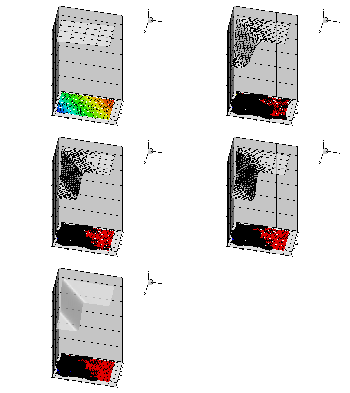
is the exact solution of the problem. The plot below shows the numerical solution for $\Phi=45^\circ$ , a Peclet number of $\mbox{Pe}= 200$ , and four different values of the "steepness parameter", $\alpha = 0.2,\ 5,\ 10$ and .

Animation of the adaptive solution for various values of the `steepness parameter'.

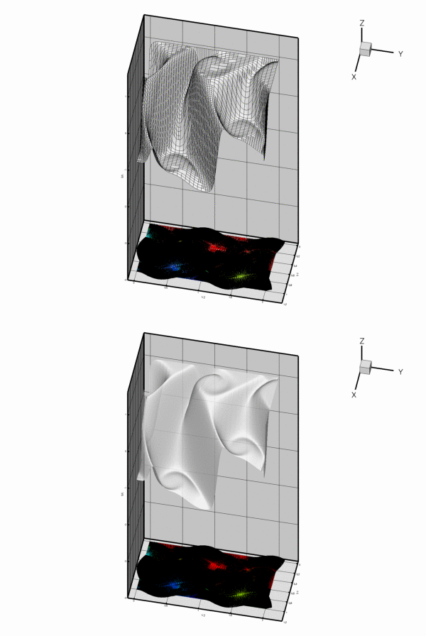
As in the example with Dirichlet boundary conditions, the unforced case is a lot more interesting. The plot below shows the result for a zero source function $f \equiv 0$ , Dirichlet boundary conditions determined from the "exact solution" of the forced problem for $\alpha = 15$ , and a prescribed flux of on $\partial D_{Neumann}$ .

Plot of the adaptive solution of the unforced problem.

Along $\partial D_{Dirichlet}$ , the value of is enforced by the Dirichlet boundary condition (2) and, as in the previous example, the "wind" either sweeps this value into the interior of the domain or creates a sharp boundary layer within which the solution that is "swept" along from the interior adjusts itself to the prescribed boundary value. Along $\partial D_{Neumann}$ , the flux boundary condition (3) imposes the normal derivative of the solution. This boundary condition is much "softer" than the Dirichlet condition and does not create boundary layers that are as sharp as the ones that develop on $\partial D_{Dirichlet}$ .

The driver code

The driver code for this problem is so similar to the corresponding Poisson problem that we do not list it here. The modifications are the same as those discussed in the advection diffusion problem with Dirichlet boundary conditions: We have to specify the wind function and the Peclet number.

Source files for this tutorial

The source files for this tutorial are located in the directory: demo_drivers/advection_diffusion/two_d_adv_diff_flux_bc/
The driver code is: demo_drivers/advection_diffusion/two_d_adv_diff_flux_bc/two_d_adv_diff_flux_bc.cc

PDF file

A pdf version of this document is available.