In this document we demonstrate the adaptive solution of the Young Laplace equation with contact angle boundary conditions. We start by reviewing the physical background in the context of a representative model problem, and then discuss the spine-based representation of free contact lines and the implementation of the contact angle boundary condition along such lines.

Acknowledgement: This tutorial and the associated driver codes were developed jointly with Cedric Ody (Ecole Polytechnique, Paris; now Rennes).

A model problem

The figure below shows a sketch of a T-junction in a microchannel with a rectangular cross-section. (The front wall has been removed for clarity). Fluid is being pushed quasi-steadily along the (vertical) main channel and is in the process of entering the T-junction. We assume that the air-liquid interface (shown in red) remains pinned at the two sharp edges (at ) where the channels meet, while the meniscus forms a quasi-static contact angle, $\gamma$ , with the smooth front and back walls.

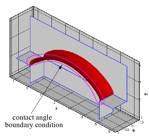
A typical problem: Fluid propagates quasi-steadily through a T-junction that connects two channels of rectangular cross-section.

It is of interest to determine the maximum pressure that the meniscus can withstand: if the driving pressure is less than that value, the fluid will not be able to propagate past the T-junction.

Theory and implementation

Spine-based representation of the meniscus

Recall that we parametrised the meniscus by two intrinsic coordinates as 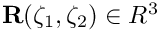${\bf R}(\zeta_1,\zeta_2) \in {R}^3$ , where 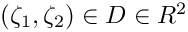$(\zeta_1,\zeta_2) \in D \in {R}^2$ . Furthermore, we parametrised the domain boundary, $\partial D$ , by a scalar coordinate $\xi$ so that,

${\partial D} = \bigg\{ (\zeta_1,\zeta_2) \ \bigg| \ (\zeta_1,\zeta_2) = \left( \zeta_1^{[\partial D]}(\xi), \ \zeta_2^{[\partial D]}(\xi) \right) \bigg\}.$

The normal to the meniscus is then given by

${\bf N} = \frac{{\bf R}_{,1} \times {\bf R}_{,2} } {|{\bf R}_{,1} \times {\bf R}_{,2}|},$

where a comma denotes partial differentiation with respect to one of the intrinsic coordinates, $(\zeta_1, \zeta_2).$

Along the contact line we define two unit vectors, ${\bf T}_t$ and ${\bf T}_n$ , that are tangential to the meniscus. ${\bf T}_t$ is tangent to the contact line while ${\bf T}_n$ is normal to it and points away from the meniscus, as shown in the sketch below.

We split the domain boundary $\partial D$ so that $\partial D = \partial D_{\rm pinned} \cup \partial D_{\rm angle}$ and assume that along $\partial D_{\rm pinned}$ the meniscus is pinned,

$\left. {\bf R} \right|_{\partial D_{\rm pinned}} = {\bf R}_{\rm pinned}(\xi),$

where ${\bf R}_{\rm pinned}(\xi)$ is given. On $\partial D_{\rm angle}$ the meniscus meets the wall at a prescribed contact angle $\gamma$ so that

$\left. \left( ({\bf T}_t \times {\bf N}_{\rm wall}) \cdot {\bf T}_n\right) \right|_{\partial D_{angle}} = \cos \gamma, \ \ \ \ \ \ \ \ \ \ \ \ \ \ \ \ \ \ \ \ \ \ (1)$

where ${\bf N}_{\rm wall}$ is the outer unit normal to the wall as shown in this sketch:

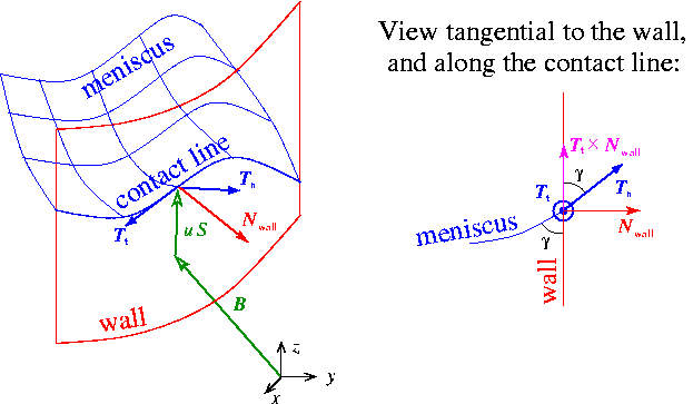
Sketch of the meniscus, the contact line along which it meets the wall, and the spine-based representation of the meniscus.

The figure also illustrates the spine-based representation of the meniscus in the form

${\bf R}(\zeta_1,\zeta_2) = {\bf B}(\zeta_1,\zeta_2) + u(\zeta_1,\zeta_2) \ {\bf S}(\zeta_1,\zeta_2) \ \ \ \ \ \ \ \ \ \ \ \ \ \ \ \ \ \ \ \ \ \ (2)$

where the spine basis ${\bf R}(\zeta_1,\zeta_2)$ and spines ${\bf S}(\zeta_1,\zeta_2)$ are pre-determined vector fields, chosen such that

The mapping from $(\zeta_1,\zeta_2)$ to ${\bf R}(\zeta_1,\zeta_2)$
is one-to-one, at least for the meniscus shapes of interest.
Along the parts of the boundary where the contact line is pinned we have
$\left. {\bf B}\right|_{\partial D_{\rm pinned}} = {\bf R}_{\rm pinned}$
so that the pinned boundary condition may be enforced by setting $u|_{\partial D_{\rm pinned}} = 0.$

Computation of the contact-angle term in the variational principle

Recall that the variational principle that determines the shape of the meniscus contained the line term

$\delta \Pi_{\rm contact \ line} = \oint_{\partial D } {\bf T}_n \cdot \delta {\bf R} \left| \frac{\partial {\bf R}} {\partial \xi}\right| \ d\xi.$

Along $\partial D_{pinned}$ the line integral vanishes because $\delta {\bf R}\big|_{ \partial D_{pinned} } ={\bf 0}$ . The line integral can therefore be written as

$\delta \Pi_{\rm contact \ line} = \int_{\partial D_{\rm angle}} {\bf T}_n \cdot \delta {\bf R} \left| \frac{\partial {\bf R}}{\partial \xi}\right| \ d\xi,$

or, using the spine-based representation of the meniscus, (2),

$\delta \Pi_{\rm contact\ line} = \int_{\partial D_{\rm angle}} {\bf T}_n \cdot {\bf S} \ \delta u \left| \frac{\partial {\bf R}}{\partial \xi}\right| \ d\xi.$

We shall now demonstrate that the integrand in this expression can be expressed in terms of the contact angle boundary condition (1). We start with several observations:

${\bf T}_t$ is tangential to the wall.
Since ${\bf N}_{\rm wall}$ is normal to the wall, ${\bf T}_t \times {\bf N}_{\rm wall}$ is tangential to the wall and orthogonal to ${\bf T}_t$ .
${\bf S}$ is tangential to the wall and can therefore be decomposed into its components parallel to ${\bf T}_t$ and ${\bf T}_t \times {\bf N}_{\rm wall}$ as
${\bf S} = \alpha {\bf T}_t + \beta ( {\bf T}_t \times {\bf N}_{\rm wall} ) \ \ \ \ \ \ \ \ \ \ \ \ \ \ \ \ \ \ \ \ (3)$
for some values of $\alpha$ and $\beta$ . In fact,
$\beta = {\bf S} \cdot ( {\bf T}_t \times {\bf N}_{\rm wall} )$
During the computation it is most convenient to perform all calculations in terms of quantities that are easily obtained from the parametrisation of the meniscus as this avoids having to specify ${\bf N}_{\rm wall}$ explicitly. For this purpose we exploit that ${\bf T}_t$ and ${\bf S}$ are tangential to the wall and not parallel to each other (unless the parametrisation of the meniscus by (2) is no longer one-to-one). Therefore ${\bf N}_{\rm wall}$ can be obtained from quantities that are intrinsic to the meniscus representation via

${\bf N}_{\rm wall} = \frac{ {\bf S} \times {\bf T}_t } {|{\bf S} \times {\bf T}_t|}$
and thus
$\beta = {\bf S} \cdot \left( {\bf T}_t \times \frac{ {\bf S} \times {\bf T}_t } {|{\bf S} \times {\bf T}_t|} \right) \ \ \ \ \ \ \ \ \ \ \ \ \ \ \ \ \ \ \ \ \ \ (4)$
Given (3) and the fact that ${\bf T}_t \cdot {\bf T}_n =0$ , we have

${\bf S} \cdot {\bf T}_n = \beta ( {\bf T}_t \times {\bf N}_{\rm wall} ) \cdot {\bf T}_n$
and with (1):
${\bf S} \cdot {\bf T}_n = \beta \cos \gamma.$
Hence, the line integral may be written as
$\delta \Pi_{\rm contact\ line} = \int_{\partial D_{\rm angle}} \beta \cos \gamma \ \delta u \left| \frac{\partial {\bf R}}{\partial \xi}\right| \ d\xi, \ \ \ \ \ \ \ \ \ \ \ \ \ \ \ \ (5)$
where $\beta$ is given by (4).

Equation (5) is easily discretised by finite elements. Within oomph-lib, the line integral is decomposed into FaceElements that are attached to the "bulk" Young-Laplace elements that are adjacent to the contact line. The imposition of the contact angle boundary condition for the Young Laplace equation is therefore as easy as the application of Neumann boundary conditions for a Poisson equation, say.

Results

The animation below illustrates the variation in the quasi-steady meniscus shape as the fluid enters the T-junction.

Animation of the meniscus shapes.

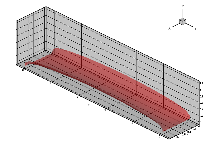
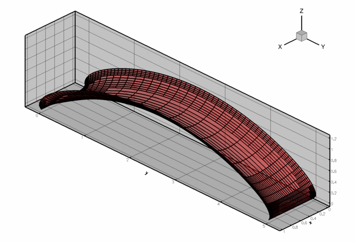
The computation was performed with full spatial adaptivity. The plot below illustrates how the automatic mesh adaptation has strongly refined the mesh towards the corners of the domain where the meniscus shape has a singularity. (The singularity develops because in the corners of the domain the contact angle boundary condition along the side walls is inconsistent with the contact angle enforced by the pinned boundary condition along the sharp edges.)

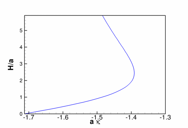
Illustration of the adaptive mesh refinement.

Finally, here is a plot of the "load-displacement diagram", i.e. a plot of the meniscus deflection as a function of its curvature (i.e. the applied pressure drop). The limit point indicates the maximum pressure that can be withstood by the static meniscus.

The load-displacement diagram for the meniscus.

The driver code

The modifications to the driver code required to impose the contact angle boundary conditions are very similar to those used in other driver codes for problems with Neumann-type boundary conditions. We attach FaceElements to the appropriate faces of the "bulk" Young-Laplace elements detach/re-attach them before and after any spatial adaptation of the "bulk" mesh.

The global namespace

The namespace that defines the problem parameters is very similar to that used in the previous example without contact angle boundary conditions. We provide storage for the cosine of the contact angle, and the prescribed meniscus height that is used by the displacement control method.

//======start_of_namespace========================================
/// Namespace for "global" problem parameters
//================================================================
namespace GlobalParameters
{
 
 /// Cos of contact angle 
 double Cos_gamma=cos(MathematicalConstants::Pi/6.0);
 
 /// Height control value for displacement control
 double Controlled_height = 0.0;

As before, we use the spine basis ${\bf B}(\zeta_1,\zeta_2)=(\zeta_1,\zeta_2,0)^T,$ to establish a reference configuration in which the flat meniscus is located in the plane and occupies the domain $(x,y) \in [0,L_x] \times [0,L_y].$

 
 /// Length of domain
 double L_x = 1.0; 
 
 /// Width of domain
 double L_y = 5.0; 
 
 // Spine basis
 //------------
 
 /// Spine basis: The position vector to the basis of the spine
 /// as a function of the two coordinates x_1 and x_2, and its
 /// derivatives w.r.t. to these coordinates. 
 /// dspine_B[i][j] = d spine_B[j] / dx_i
 /// Spines start in the (x_1,x_2) plane at (x_1,x_2).
 void spine_base_function(const Vector<double>& x, 
                          Vector<double>& spine_B, 
                          Vector< Vector<double> >& dspine_B)
 {
  
  // Bspines and derivatives 
  spine_B[0]     = x[0];
  spine_B[1]     = x[1];
  spine_B[2]     = 0.0 ;
  dspine_B[0][0] = 1.0 ;
  dspine_B[1][0] = 0.0 ;
  dspine_B[0][1] = 0.0 ; 
  dspine_B[1][1] = 1.0 ;
  dspine_B[0][2] = 0.0 ;
  dspine_B[1][2] = 0.0 ;
  
 } // End of bspine functions

As in the previous example, we rotate the spines in the -direction to allow the representation of meniscus shapes that cannot be projected onto the -plane.

 
 
 
 // Spines rotate in the y-direction
 //---------------------------------
 
 /// Min. spine angle against horizontal plane
 double Alpha_min = MathematicalConstants::Pi/2.0*1.5;
 
 /// Max. spine angle against horizontal plane
 double Alpha_max = MathematicalConstants::Pi/2.0*0.5;
 
 /// Spine: The spine vector field as a function of the two 
 /// coordinates x_1 and x_2, and its derivatives w.r.t. to these coordinates:
 /// dspine[i][j] = d spine[j] / dx_i
 void spine_function(const Vector<double>& x, 
                     Vector<double>& spine, 
                     Vector< Vector<double> >& dspine)
 {
  
  /// Spines (and derivatives)  are independent of x[0] and rotate 
  /// in the x[1]-direction
  spine[0]=0.0;
  dspine[0][0]=0.0; 
  dspine[1][0]=0.0; 
  
  spine[1]=cos(Alpha_min+(Alpha_max-Alpha_min)*x[1]/L_y); 
  dspine[0][1]=0.0;                                   
  dspine[1][1]=-sin(Alpha_min+(Alpha_max-Alpha_min)*x[1]/L_y)
   *(Alpha_max-Alpha_min)/L_y;            
  
  spine[2]=sin(Alpha_min+(Alpha_max-Alpha_min)*x[1]/L_y);
  dspine[0][2]=0.0;                                  
  dspine[1][2]=cos(Alpha_min+(Alpha_max-Alpha_min)*x[1]/L_y) 
   *(Alpha_max-Alpha_min)/L_y;            
 
 } // End spine function
 
 
} // end of namespace

The driver code

We start by defining the output directory and open a trace file to record the load-displacement curve.

//===============start_of_main============================================
/// Drive code
//========================================================================
int main()
{
 
 // Create label for output
 DocInfo doc_info;
 
 // Trace file
 ofstream trace_file;
 
 // Set output directory
 doc_info.set_directory("RESLT");
 
 // Open a trace file
 char filename[100];
 sprintf(filename,"%s/trace.dat",doc_info.directory().c_str());
 trace_file.open(filename);
 
 // Tecplot header for trace file: kappa and height value
 trace_file << "VARIABLES=\"<GREEK>k</GREEK>\",\"h\"" << std::endl;
 trace_file << "ZONE" << std::endl;

Next, we create the problem object, refine the mesh uniformly and output the initial guess for the solution: a flat interface which, unlike the previous case, is not a solution of the problem because it does not satisfy the contact-angle boundary condition; see the section Comments and Exercises for a more detailed discussion of this issue.

 
 
 //Set up the problem
 //------------------
 
 // Create the problem with 2D nine-node elements from the
 // RefineableQYoungLaplaceElement family. 
 RefineableYoungLaplaceProblem<RefineableQYoungLaplaceElement<3> > problem;
 
 // Perform one uniform refinement
 problem.refine_uniformly();
 
 //Output the solution
 problem.doc_solution(doc_info,trace_file);
 
 //Increment counter for solutions 
 doc_info.number()++;

Finally, we perform a parameter study by slowly incrementing the control displacement and recomputing the meniscus shape.

 
 // Parameter incrementation
 //------------------------- 
 double increment=0.1;
 
 // Loop over steps
 unsigned nstep=2; // 10;
 for (unsigned istep=0;istep<nstep;istep++)
  {
   GlobalParameters::Controlled_height+=increment;
 
   // Solve the problem  
   unsigned max_adapt=1;
   problem.newton_solve(max_adapt);
 
   //Output the solution
   problem.doc_solution(doc_info,trace_file);
   
   //Increment counter for solutions 
   doc_info.number()++;
  }
 
 // Close output file
 trace_file.close();
 
} //end of main

The problem class

The problem class contains the usual member functions. The functions actions_before_adapt() and actions_after_adapt() are used to detach and re-attach (and rebuild) the contact angle elements on the appropriate boundaries of the "bulk" mesh.

//====== start_of_problem_class=======================================
/// 2D RefineableYoungLaplace problem on rectangular domain, discretised with
/// 2D QRefineableYoungLaplace elements. The specific type of element is
/// specified via the template parameter.
//====================================================================
template<class ELEMENT> 
class RefineableYoungLaplaceProblem : public Problem
{
 
public:
 
 /// Constructor: 
 RefineableYoungLaplaceProblem();
 
 /// Destructor (empty)
 ~RefineableYoungLaplaceProblem(){};
 
 /// Update the problem specs before solve: Empty
 void actions_before_newton_solve(){};
 
 /// Update the problem after solve: Empty
 void actions_after_newton_solve(){};
 
 /// Actions before adapt: Wipe the mesh of contact angle elements
 void actions_before_adapt()
  {
   // Kill the contact angle elements and wipe contact angle mesh
   if (Contact_angle_mesh_pt!=0) delete_contact_angle_elements();
 
   // Rebuild the Problem's global mesh from its various sub-meshes
   rebuild_global_mesh();
  }
 
 
 ///  Actions after adapt: Rebuild the mesh of contact angle elements
 void actions_after_adapt()
  {
   create_contact_angle_elements(1);
   create_contact_angle_elements(3);
   
   // Set function pointers for contact-angle elements
   unsigned nel=Contact_angle_mesh_pt->nelement();
   for (unsigned e=0;e<nel;e++)
    {
     // Upcast from GeneralisedElement to YoungLaplace contact angle
     // element
     YoungLaplaceContactAngleElement<ELEMENT> *el_pt = 
      dynamic_cast<YoungLaplaceContactAngleElement<ELEMENT>*>(
       Contact_angle_mesh_pt->element_pt(e));
     
     // Set the pointer to the prescribed contact angle
     el_pt->prescribed_cos_gamma_pt() = &GlobalParameters::Cos_gamma;
    }
   
   // Rebuild the Problem's global mesh from its various sub-meshes
   rebuild_global_mesh();
   
  }
 
 /// Doc the solution. DocInfo object stores flags/labels for where the
 /// output gets written to and the trace file
 void doc_solution(DocInfo& doc_info, ofstream& trace_file);

Two private helper functions are provided to create and delete the contact angle elements. The class also provides storage for the pointers to the various meshes, to the node at which the meniscus displacement is prescribed by the displacement control method, and to the Data object whose one-and-only value stores the (unknown) meniscus curvature.

 
private:
 
 /// Create YoungLaplace contact angle elements on the 
 /// b-th boundary of the bulk mesh and add them to contact angle mesh
 void create_contact_angle_elements(const unsigned& b);
 
 /// Delete contact angle elements 
 void delete_contact_angle_elements();
 
 /// Pointer to the "bulk" mesh
 RefineableRectangularQuadMesh<ELEMENT>* Bulk_mesh_pt;
 
 /// Pointer to the contact angle mesh
 Mesh* Contact_angle_mesh_pt;
 
 /// Pointer to mesh containing the height control element
 Mesh* Height_control_mesh_pt;
 
 /// Node at which the height (displacement along spine) is controlled/doced
 Node* Control_node_pt;
 
 /// Pointer to Data object that stores the prescribed curvature
 Data* Kappa_pt;
 
}; // end of problem class

The problem constructor

We start by creating the "bulk" mesh of refineable Young Laplace elements and specify the error estimator.

//=====start_of_constructor===============================================
/// Constructor for RefineableYoungLaplace problem
//========================================================================
template<class ELEMENT>
RefineableYoungLaplaceProblem<ELEMENT>::RefineableYoungLaplaceProblem()
{ 
 
 // Setup bulk mesh
 //----------------
 
 // # of elements in x-direction
 unsigned n_x=8;
 
 // # of elements in y-direction
 unsigned n_y=8;
 
 // Domain length in x-direction
 double l_x=GlobalParameters::L_x;
 
 // Domain length in y-direction
 double l_y=GlobalParameters::L_y;
 
 // Build and assign mesh
 Bulk_mesh_pt=new RefineableRectangularQuadMesh<ELEMENT>(n_x,n_y,l_x,l_y);
 
 // Create/set error estimator
 Bulk_mesh_pt->spatial_error_estimator_pt()=new Z2ErrorEstimator;
 
 // Set targets for spatial adaptivity
 Bulk_mesh_pt->max_permitted_error()=1.0e-4;
 Bulk_mesh_pt->min_permitted_error()=1.0e-6;

We identify the node (in the centre of the mesh) at which we apply displacement control. We pass a pointer to this node to the constructor of the displacement control element and store that element in its own mesh.

 
 // Check that we've got an even number of elements otherwise
 // out counting doesn't work...
 if ((n_x%2!=0)||(n_y%2!=0))
  {
   cout << "n_x n_y should be even" << endl;
   abort();
  }
  
 //  This is the element that contains the central node:
 ELEMENT* prescribed_height_element_pt= dynamic_cast<ELEMENT*>(
  Bulk_mesh_pt->element_pt(n_y*n_x/2+n_x/2));
 
 // The central node is node 0 in that element
 Control_node_pt= static_cast<Node*>(prescribed_height_element_pt->node_pt(0));
 
 std::cout << "Controlling height at (x,y) : (" << Control_node_pt->x(0) 
           << "," << Control_node_pt->x(1)  << ")" << "\n" << endl;
 
 // Create a height control element and store the
 // pointer to the Kappa Data created by this object
 HeightControlElement* height_control_element_pt=new HeightControlElement(
  Control_node_pt,&GlobalParameters::Controlled_height);
 
 // Add to mesh
 Height_control_mesh_pt = new Mesh;
 Height_control_mesh_pt->add_element_pt(height_control_element_pt);
 
 // Store curvature data
 Kappa_pt=height_control_element_pt->kappa_pt();

Next we create the mesh that stores the contact-angle elements. We attach these elements to boundaries 1 and 3 of the "bulk" mesh.

 
 
 // Contact angle elements
 //-----------------------
 
 // Create prescribed-contact-angle elements from all elements that are 
 // adjacent to boundary 1 and 3 and add them to their own mesh
 
 // set up new mesh
 Contact_angle_mesh_pt=new Mesh;
 
 // creation of contact angle elements
 create_contact_angle_elements(1);
 create_contact_angle_elements(3);

The various sub-meshes are now added to the problem and the global mesh is built.

 
 
 // Add various meshes and build the global mesh
 //----------------------------------------------
 add_sub_mesh(Bulk_mesh_pt);
 add_sub_mesh(Height_control_mesh_pt);
 add_sub_mesh(Contact_angle_mesh_pt);
 build_global_mesh();

As usual, we enforce only the essential boundary conditions directly by pinning the meniscus displacement along mesh boundaries 0 and 2:

 
 
 // Boundary conditions
 //--------------------
 
 // Set the boundary conditions for this problem: All nodes are
 // free by default -- only need to pin the ones that have Dirichlet conditions
 // here. 
 unsigned n_bound = Bulk_mesh_pt->nboundary(); 
 for(unsigned b=0;b<n_bound;b++)
  {
   // Pin all boundaries for three cases and only boundaries
   // 0 and 2 in all others:
   if ((b==0)||(b==2))
    {
     unsigned n_node = Bulk_mesh_pt->nboundary_node(b);
     for (unsigned n=0;n<n_node;n++)
      {
       Bulk_mesh_pt->boundary_node_pt(b,n)->pin(0); 
      }
    }
  } // end bcs

The build of the "bulk" Young Laplace elements is completed by specifying the function pointers to the spine functions and the pointer to the Data object that stores the curvature.

 
 // Complete build of elements
 //---------------------------
 
 // Complete the build of all elements so they are fully functional 
 unsigned n_bulk=Bulk_mesh_pt->nelement();
 for(unsigned i=0;i<n_bulk;i++)
  {
   // Upcast from GeneralsedElement to the present element
   ELEMENT *el_pt = dynamic_cast<ELEMENT*>(Bulk_mesh_pt->element_pt(i));
 
   //Set the spine function pointers
   el_pt->spine_base_fct_pt() = GlobalParameters::spine_base_function;
   el_pt->spine_fct_pt() =  GlobalParameters::spine_function;
  
   // Set the curvature data for the element
   el_pt->set_kappa(Kappa_pt); 
  }

Finally, we complete the build of the contact line elements by passing the pointer to the double that stores the cosine of the contact angle.

 
 // Set function pointers for contact-angle elements
 unsigned nel=Contact_angle_mesh_pt->nelement();
 for (unsigned e=0;e<nel;e++)
  {
   // Upcast from GeneralisedElement to YoungLaplace contact angle 
   // element
   YoungLaplaceContactAngleElement<ELEMENT> *el_pt = 
    dynamic_cast<YoungLaplaceContactAngleElement<ELEMENT>*>(
     Contact_angle_mesh_pt->element_pt(e));
   
   // Set the pointer to the prescribed contact angle
   el_pt->prescribed_cos_gamma_pt() = &GlobalParameters::Cos_gamma;
  }

All that's now left to do is to assign the equation numbers:

 
 // Setup equation numbering scheme
 cout <<"\nNumber of equations: " << assign_eqn_numbers() << endl; 
 cout << "\n********************************************\n" <<  endl;
 
} // end of constructor

Creating the contact angle elements

The function create_contact_angle_elements() attaches the FaceElements that apply the contact angle boundary condition to the specified boundary of the "bulk" mesh. Pointers to the newly-created FaceElements are stored in a separate mesh.

//============start_of_create_contact_angle_elements=====================
/// Create YoungLaplace contact angle elements on the b-th boundary of the 
/// bulk mesh and add them to the contact angle mesh
//=======================================================================
template<class ELEMENT>
void RefineableYoungLaplaceProblem<ELEMENT>::create_contact_angle_elements(
 const unsigned &b)
{
 // How many bulk elements are adjacent to boundary b?
 unsigned n_element = Bulk_mesh_pt->nboundary_element(b);
 
 // Loop over the bulk elements adjacent to boundary b?
 for(unsigned e=0;e<n_element;e++)
  {
   // Get pointer to the bulk element that is adjacent to boundary b
   ELEMENT* bulk_elem_pt = dynamic_cast<ELEMENT*>(
    Bulk_mesh_pt->boundary_element_pt(b,e));
 
   // What is the index of the face of the bulk element at the boundary
   int face_index = Bulk_mesh_pt->face_index_at_boundary(b,e);
   
   // Build the corresponding contact angle element
   YoungLaplaceContactAngleElement<ELEMENT>* contact_angle_element_pt = new 
   YoungLaplaceContactAngleElement<ELEMENT>(bulk_elem_pt,face_index);
 
   //Add the contact angle element to the contact angle mesh
   Contact_angle_mesh_pt->add_element_pt(contact_angle_element_pt);
 
  } //end of loop over bulk elements adjacent to boundary b
 
} // end of create_contact_angle_elements

Deleting the contact angle elements

The function delete_contact_angle_elements() deletes the contact angle elements and flushes the associated mesh.

//============start_of_delete_contact_angle_elements=====================
/// Delete YoungLaplace contact angle elements
//=======================================================================
template<class ELEMENT>
void RefineableYoungLaplaceProblem<ELEMENT>::delete_contact_angle_elements()
{
 
 // How many contact angle elements are there?
 unsigned n_element = Contact_angle_mesh_pt->nelement();
 
 // Loop over the surface elements
 for(unsigned e=0;e<n_element;e++)
  {
   // Kill surface element
   delete Contact_angle_mesh_pt->element_pt(e);
  }
 
 // Wipe the mesh
 Contact_angle_mesh_pt->flush_element_and_node_storage();
 
 
} // end of delete_contact_angle_elements

Post-processing

We output the load-displacement data, the meniscus shape, and various contact line quantities.

//===============start_of_doc=============================================
/// Doc the solution: doc_info contains labels/output directory etc.
//========================================================================
template<class ELEMENT>
void RefineableYoungLaplaceProblem<ELEMENT>::doc_solution(DocInfo& doc_info,
                                              ofstream& trace_file)
{ 
 
 // Output kappa vs height
 //-----------------------
 trace_file << -1.0*Kappa_pt->value(0) << " ";
 trace_file << Control_node_pt->value(0) ;
 trace_file << endl;
  
 // Number of plot points: npts x npts
 unsigned npts=5;
 
 // Output full solution 
 //---------------------
 ofstream some_file;
 char filename[100];
 //YoungLaplaceEquations::Output_meniscus_and_spines=false;
 sprintf(filename,"%s/soln%i.dat",doc_info.directory().c_str(),
         doc_info.number());
 some_file.open(filename);
 Bulk_mesh_pt->output(some_file,npts);
 some_file.close();
 
 // Output contact angle 
 //---------------------
 
 ofstream tangent_file;
 sprintf(filename,"%s/tangent_to_contact_line%i.dat",
         doc_info.directory().c_str(),
         doc_info.number());
 tangent_file.open(filename);
 
 ofstream normal_file;
 sprintf(filename,"%s/normal_to_contact_line%i.dat",
         doc_info.directory().c_str(),
         doc_info.number());
 normal_file.open(filename);
 
 
 ofstream contact_angle_file;
 sprintf(filename,"%s/contact_angle%i.dat",
         doc_info.directory().c_str(),
         doc_info.number());
 contact_angle_file.open(filename);
 
 // Tangent and normal vectors to contact line
 Vector<double> tangent(3);
 Vector<double> normal(3);
 Vector<double> r_contact(3);
 
 // How many contact angle elements are there?
 unsigned n_element = Contact_angle_mesh_pt->nelement();
 
 // Loop over the surface elements
 for(unsigned e=0;e<n_element;e++)
  {
   
   tangent_file << "ZONE" << std::endl;
   normal_file << "ZONE" << std::endl;
   contact_angle_file << "ZONE" << std::endl;
   
   // Upcast from GeneralisedElement to YoungLaplace contact angle element
   YoungLaplaceContactAngleElement<ELEMENT>* el_pt = 
    dynamic_cast<YoungLaplaceContactAngleElement<ELEMENT>*>(
     Contact_angle_mesh_pt->element_pt(e));
   
   // Loop over a few points in the contact angle element
   Vector<double> s(1);
   for (unsigned i=0;i<npts;i++)
    {
     s[0]=-1.0+2.0*double(i)/double(npts-1);
     
     dynamic_cast<ELEMENT*>(el_pt->bulk_element_pt())->
      position(el_pt->local_coordinate_in_bulk(s),r_contact);
     
     el_pt->contact_line_vectors(s,tangent,normal);
     tangent_file << r_contact[0] << " " 
                  << r_contact[1] << " " 
                  << r_contact[2] << " " 
                  << tangent[0] << " " 
                  << tangent[1] << " " 
                  << tangent[2] << " "  << std::endl;
     
     normal_file << r_contact[0] << " " 
                 << r_contact[1] << " " 
                 << r_contact[2] << " " 
                 << normal[0] << " " 
                 << normal[1] << " " 
                 << normal[2] << " "  << std::endl;
     
     contact_angle_file << r_contact[1] << " " 
                        << el_pt->actual_cos_contact_angle(s)
                        << std::endl;
    }
   
   
  } // end of loop over both boundaries
 
 tangent_file.close();
 normal_file.close();
 contact_angle_file.close();
 
 
cout << "\n********************************************" << endl <<  endl;
 
} // end of doc

Comments and Exercises

How to generate a good initial guess for the solution

We already commented on the need to provide a "good" initial guess for the solution in order to ensure the convergence of the Newton iteration. In the previous example this was easy because the flat meniscus (clearly a solution of the Young-Laplace equations for zero curvature) also satisfied the boundary conditions. In the present example, and in many others, this is not the case. In such problems it may be difficult to generate initial guesses for the meniscus shape that are sufficiently close to actual solution.

In such cases it may be necessary to compute the initial solution to the problem whose behaviour we wish to investigate during the actual parameter study via a preliminary auxiliary continuation procedure that transforms an easier-solve-problem (for which a good initial guess can be found) into the actual problem.

Explore this approach in the present problem by implementing the following steps:

Set the contact angle to and solve the problem, using the "flat" meniscus as the initial guess. The "flat" meniscus is, of course, the exact solution for zero control displacement and/or zero curvature.
Now start a preliminary continuation procedure in which the contact angle is adjusted in small steps until it reaches the desired value. Keep the prescribed control displacement (or the meniscus curvature) constant during this procedure.
The solution for the desired contact angle may now be used as the initial guess for the actual parameter study in which the control displacement (or the meniscus curvature) are increased while the contact angle is kept fixed.

Limitations of the current approach – suggestions for improvement

One of the main disadvantages of the approach adopted here is that the spine vector fields ${\bf B}$ and ${\bf S}$ must be specified a priori. For sufficiently complicated meniscus shapes (or for menisci that undergo large changes in shape as their curvature is varied) the choice of suitable spines may be very difficult.

One (possible) solution to this problem could be (we haven't tried it!) to occasionally update the spine representation. For instance, assume that we have computed a meniscus shape in the form

$\widehat{\bf R} = {\bf R}(\zeta_1,\zeta_2) = {\bf B}(\zeta_1,\zeta_2) + u(\zeta_1,\zeta_2) \ {\bf S}(\zeta_1,\zeta_2)$

with an associated normal vector $\widehat{\bf N}$ . We can reparametrise this shape by setting

${\bf B} := \widehat{\bf R},$

${\bf S} := \widehat{\bf N},$

and

$u := 0$

before continuing the computation. Provided this is done sufficiently frequently, i.e. long before the displacement along the spines has become so large that the mapping from $(\zeta_1,\zeta_2)$ to ${\bf R}(\zeta_1,\zeta_2)$ is about to become non-one-to-one, this should allow the computation of arbitrarily large meniscus deflections. Try it out and let us know how it works!

Zero contact angles

Our problem formulation suffers from an additional, more fundamental problem: it cannot be used to solve problems with zero contact angle. This is because for zero contact angles the equilibrium solution is no longer a minimiser of the variational principle: given a solution at which the meniscus meets the wall at zero contact angle, it is always possible to extend the meniscus with an arbitrary-length "collar" along the wall without changing the overall energy of the system. As a result, the position of the contact line becomes increasingly ill-defined as the contact angle $\gamma$ is reduced, causing the Newton method to converge very slowly (and ultimately not at all) as $\gamma \to 0.$

Source files for this tutorial

The source files for this tutorial are located in the directory:

demo_drivers/young_laplace/
The driver code is:

demo_drivers/young_laplace/refineable_t_junction.cc

PDF file

A pdf version of this document is available.