Overview of the problem

We consider an open rectangular container of unit width containing a still viscous fluid of prescribed volume $\mathcal{V}$ that meets the wall of the container at a contact angle $\theta_{c}$ . The external fluid is assumed to be inviscid and massless and acts only through an external pressure, $P_{\mbox{ext}}$ , at the bounding (free) surface of the viscous fluid. In the absence of any body forces or external forcing, a static solution is obtained in which the velocity field is zero, the fluid pressure is a constant, $P_{\mbox{fluid}}$ , and free surface is of constant curvature (an arc of a circle in two-dimensions), set by the contact angle and the geometry of the domain. From simple geometry, the mean curvature of the interface in the present problem is 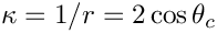$\kappa = 1/r = 2\cos\theta_{c}$ , see the figure below. The pressure difference across the interface, $\Delta P = P_{\mbox{ext}} - P_{\mbox{fluid}}$ , then follows from the dynamic boundary condition.

Sketch of the problem: the static interface curvature is set by the geometry

The governing equations are the Navier–Stokes equations together with the free surface boundary conditions at the upper surface, see another tutorial for further details. As in that tutorial, we also compute the deformation of the internal fluid mesh by using a pseudo-solid node-update strategy.

For simplicity, we assume symmetry of the domain about the vertical centreline of the container, which we choose to be the $x_{2}$ -axis; hence, the initial computational domain is $x_{1} \in [0,0.5],\ x_{2} \in [0,1]$ . The fluid boundary conditions are no slip, $u_{i} = 0$ , on the container boundaries at $x_{2} =0$ and $x_{1} = 0.5;$ and a symmetry condition at $x_{1} = 0$ . Under the standard non-dimensionalisation the pressure difference over the interface is 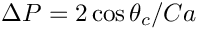$\Delta P = 2\cos\theta_{c}/Ca$ , where is the capillary number, also defined in the other tutorial. In the present (static) example, the capillary number is a simple multiplicative factor that sets the pressure scale.

There remain the two additional constraints that must be enforced:

The fluid volume must be $\mathcal{V}$ .
The contact angle where the fluid meets the container wall at $x_{1} = 0.5$ must be $\theta_{c}.$

Enforcing the volume constraint

For capillary-static problems, the fluid velocity field is zero and the continuity equation 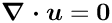$\mbox{\boldmath$\nabla\cdot u$} = \mbox{\boldmath$0$}$ is trivially satisfied. Thus, conservation of mass is not guaranteed without an additional constraint. Mathematically speaking, the system is underdetermined and the equation associated with a pressure degree of freedom (either a fluid pressure or the external pressure) can be replaced by the additional volume constraint, specified by the equation:

$\frac{1}{2} \oint \mbox{\boldmath$x\cdot n$} \mbox{d} s = \frac{1}{2} \int \hspace{-0.25cm} \int \mbox{\boldmath$\nabla\cdot x$} \mbox{d} A = \int \hspace{-0.25cm} \int \mbox{d} A = \mathcal{V}.$

MATTHIAS, see also the droplet/bubble problems.

Perhaps the most natural implementation in the present problem is to fix a reference pressure value within the fluid and then to treat the external pressure as a degree of freedom with the volume constraint as the associated equation. Alternatively, the external pressure can be fixed at a reference pressure and an internal fluid pressure degree of freedom is then associated with the volume constraint. We shall demonstrate both methods in the driver code below.

Computation of the above equation associated with the volume constraint is performed by specialised LineVolumeConstraintBoundingElements that must be attached to all boundaries that enclose the fluid.

Enforcing the contact angle constraint

Here the `‘natural’' contact-angle boundary condition arises from the weak form of the dynamic boundary condition after integration using the surface divergence theorem. This leads to a term of the form

$\frac{1}{Ca} \left[m_{i}\psi\right]_{\mbox{\boldmath$x$}_l}^{\mbox{\boldmath$x$}_{r}}$

in the momentum equations associated with the boundaries of the free surface, where $\mbox{\boldmath$m$}$ is a unit vector tangential to the free surface at those boundaries.

At the (left-hand) symmetry boundary, $\mbox{\boldmath$x$}_{l}$ , we neglect this additional term in the momentum equation associated with the tangential direction, which ensures that the interface is (weakly) normal to the symmetry boundary. At the (right-hand) container boundary, $\mbox{\boldmath$x$}_{r}$ , the contact angle could be enforced by adding a boundary term with prescribed $\mbox{\boldmath$m$}$ . In general,

$\mbox{\boldmath$m$} = \cos\theta_{c} \mbox{\boldmath$n$}_{w} + \sin\theta_{c} \mbox{\boldmath$t$}_{w},$

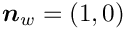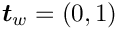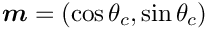where $\mbox{\boldmath$n$}_{w}$ is the normal vector to the bounding wall directed out of the fluid and $\mbox{\boldmath$t$}_{w}$ is the tangent vector to the wall. In the present example, $\mbox{\boldmath$n$}_{w} = (1,0)$ and $\mbox{\boldmath$t$}_{w} = (0,1)$ , which gives $\mbox{\boldmath$m$} = (\cos\theta_{c}, \sin\theta_{c})$ .

Unfortunately, the no-slip boundary condition at the wall means that the momentum equation is not assembled at the interface boundaries. If we wanted to use this method of (weak) enforcement of the contact angle condition, the velocity degrees of freedom at the node on the right-hand end of the free surface must be unpinned, but the no-slip condition will then not be imposed. In fact, this problem is deeper than it might appear and is a manifestation of the failure of the continuum hypothesis to treat dynamic (moving) contact lines. The correct (mathematical) treatment of that problem is still unresolved, but in this static problem, there is an alternative treatment.

Here, we can make use of the fact that the kinematic condition is also trivially satisfied because the velocity field is zero. Thus, we replace the kinematic condition associated with the right-most node on the interface by the (strong) condition that

$\cos\theta_{c} = \mbox{\boldmath$n\cdot n$}_{w},$

where $\mbox{\boldmath$n$}$ is the outer unit normal to the free surface and $\mbox{\boldmath$n$}_{w}$ is the unit normal to the bounding wall directed out of the fluid, as before.

The imposition of the contact angle condition is implemented within FluidInterfaceBoundingElements that are FaceElements of the FluidInterfaceElements; in other words, they are elements that are two spatial dimensions lower than the bulk elements. In two-dimensional problems, the FluidInterfaceBoundingElement's are PointElements.

Problem Parameters

We use a namespace to define the parameters for the pseudo-solid mesh constitutive law used in the problem and a function that defines the outer unit normal to the container boundary which is . The other problem parameters: the contact angle, prescribed volume and capillary number, are specified as member data of the problem class, see below, so that they will be re-initialised when different instances of the class are constructed.

//====start_of_namespace=================================
/// Namespace for phyical parameters
//=======================================================
namespace Global_Physical_Variables
{
 
 /// Pseudo-solid Poisson ratio
 double Nu=0.1;
 
 /// Direction of the wall normal vector
 Vector<double> Wall_normal;
 
 /// Function that specifies the wall unit normal
 void wall_unit_normal_fct(const Vector<double> &x, 
                      Vector<double> &normal)
 {
  normal=Wall_normal;
 }
 
} //end_of_namespace

The driver code

We shall solve the problem twice, once using the external pressure as the degree of freedom associated with the volume constraint and once using an internal fluid pressure degree of freedom instead. The choice of which degree of freedom to use is determined by the boolean flag passed to the problem constructor. The driver consists of a simple loop to cover both possibilities, construction of the problem and then a call to run the parameter study with different output directories in each case.

//===start_of_main=======================================================
/// Main driver: Build problem and initiate parameter study
//======================================================================
int main()
{
  // Solve the pseudosolid problem twice, once hijacking an internal, once
 // hijacking the external pressure
 for (unsigned i=0;i<2;i++)
  {
   bool hijack_internal=false;
   if (i==1) hijack_internal=true;
   //Construct the problem
   PseudoSolidCapProblem<Hijacked<
     PseudoSolidNodeUpdateElement<QCrouzeixRaviartElement<2>,
    QPVDElementWithPressure<2> > > >  problem(hijack_internal);
 
   string dir_name="RESLT_elastic_hijacked_external";
   if (i==1) dir_name="RESLT_elastic_hijacked_internal";
 
   //Do parameter study
   problem.parameter_study(dir_name);
  }
 
} //end_of_main

The elements are Hijacked PseudoSolidNodeUpdate QCrouzeixRaviart type elements, where the Hijacked actually required only in the case when an internal pressure degree of freedom is to be used to enforce the volume constraint, see below.

The problem class

The problem class consists of a constructor that takes the aforementioned boolean flag to determine which pressure degree of freedom to use for the volume constraint; a destructor to clean up all memory allocated during the problem construction; a function that performs a parameter study, decreasing the contact angle from $\theta_{c} = 90^{\circ}$ in steps of $5^{\circ}$ ; and a function that documents the solution.

//===========start_of_pseudo_elastic_class====================================
/// A class that solves the Navier--Stokes equations
/// to compute the shape of a static interface in a rectangular container
/// with imposed contact angle at the boundary.
//============================================================================
template<class ELEMENT>
class PseudoSolidCapProblem : public Problem
{
public:
 
 /// Constructor: Boolean flag indicates if volume constraint is
 /// applied by hijacking internal or external pressure
 PseudoSolidCapProblem(const bool& hijack_internal);
 
 /// Destructor: clean up memory allocated by the object
 ~PseudoSolidCapProblem();
 
 /// Peform a parameter study: Solve problem for a range of contact angles
 /// Pass name of output directory as a string
 void parameter_study(const string& dir_name);
 
 /// Doc the solution
 void doc_solution(DocInfo& doc_info);

There are also three helper functions that are used to create the FaceElements used to enforce the additional boundary conditions and constraints. The function create_free_surface_elements() adds ElasticLineFluidInterfaceElements to the upper boundary (boundary 2) of the mesh, exactly as in another tutorial . The function create_volume_constraint_elements() constructs the elements required to enforce the volume constraint. Finally, the function create_contact_angle_element() constructs the PointElement that enforces the contact angle condition at the solid wall of the container.

 
private:
 
 /// Create the free surface elements
 void create_free_surface_elements();
 
 /// Create the volume constraint elements
 void create_volume_constraint_elements();
 
 /// Create the contact angle element
 void create_contact_angle_element();

Finally, the class has member data corresponding to the physical variables of the problem and provides permanent storage for pointers to the data that stores the external pressure and the data for the pressure degree of freedom that will be "traded" for the volume constraint. In additional, an output stream and pointers to the different meshes that will be assembled in the problem are also included.

 
 /// The Capillary number 
 double Ca;
 
 /// The prescribed volume of the fluid
 double Volume;
 
 /// The external pressure
 double Pext;
 
 /// The contact angle
 double Angle;
 
 /// Constitutive law used to determine the mesh deformation
 ConstitutiveLaw *Constitutive_law_pt;
 
 /// Data object whose single value stores the external pressure
 Data* External_pressure_data_pt;
 
 // Pointer to the (single valued) Data item that
 // will contain the pressure value that we're
 // trading for the volume constraint
 Data* Traded_pressure_data_pt;
 
 /// Trace file
 ofstream Trace_file;
 
 /// Storage for the bulk mesh
 Mesh* Bulk_mesh_pt;
 
 /// Storage for the free surface mesh
 Mesh* Free_surface_mesh_pt;
 
 /// Storage for the element bounding the free surface
 Mesh* Free_surface_bounding_mesh_pt;
 
 /// Storage for the elements that compute the enclosed volume
 Mesh* Volume_computation_mesh_pt;
 
 /// Storage for the volume constraint
 Mesh* Volume_constraint_mesh_pt;
 
}; //end_of_pseudo_solid_problem_class

The problem constructor

The constructor first initialises the member data and sets the outer unit normal to the wall to be . The initial contact angle is set to be $90^{\circ}$ , so that the interface will be horizontal.

//============start_of_constructor=====================================
/// Constructor: Pass boolean flag to indicate if the volume
/// constraint is applied by hijacking an internal pressure
/// or the external pressure
//======================================================================
template<class ELEMENT>
PseudoSolidCapProblem<ELEMENT>::PseudoSolidCapProblem(const bool& hijack_internal) :
 Ca(2.1),       //Initialise value of Ca to some random value
 Volume(0.5),   //Initialise the value of the volume 
 Pext(1.23),    //Initialise the external pressure to some random value
 Angle(0.5*MathematicalConstants::Pi) //Initialise the contact angle
{
 //Set the wall normal
 Global_Physical_Variables::Wall_normal.resize(2);
 Global_Physical_Variables::Wall_normal[0] = 1.0; 
 Global_Physical_Variables::Wall_normal[1] = 0.0;

Next, a $4 \times 4$ element rectangular mesh is constructed on the undeformed domain.

 
 // Number of elements in the horizontal direction
 unsigned nx=4;
 
 // Number of elements in the vertical direction
 unsigned nh=4;
 
 // Halfwidth of domain
 double half_width=0.5;
 
 //Construct mesh
 Bulk_mesh_pt = new ElasticRectangularQuadMesh<ELEMENT>(nx,nh,half_width,1.0);

A Data object containing a single value is constructed to store the external pressure and the initial value is set.

 
 //Create a Data object whose single value stores the
 //external pressure
 External_pressure_data_pt = new Data(1);
 
 // Set external pressure
 External_pressure_data_pt->set_value(0,Pext);

We next setup the reference pressure and traded pressure. If we are using the external pressure as the reference pressure, then we pin it and set an internal pressure degree of freedom as the "traded" pressure. In order to use an internal pressure degree of freedom as the "traded" pressure, we must ensure that the original associated (continuity) equation is not assembled, but that the degree of freedom is still treated a fluid pressure variable when assembling the other residuals within the element. In addition, we will also need direct access to the data and its global equation number. The appropriate machinery is provided by the Hijacked wrapper class which allows variables within an underlying element to be "hijacked". The bulk elements are of QCrouzeixRaviart type, which means that the pressure variables are internal data and we hijack the first of these in the first element (although any would do). The function hijack_internal_value(..) instructs the bulk element to null out any contributions to the residuals and Jacobian matrix associated with that global equation number and returns a "custom" Data object that consists of a single value corresponding to the "hijacked" value and its global equation number. The "custom" Data object can then be used as external data in other elements that assemble the new residuals. It is important that any hijacked degrees of freedom must have residual contributions provided by another element otherwise the system Jacobian matrix will be singular. For more details about "hijacking" see this document.

 
 // Which pressure are we trading for the volume constraint: We 
 // can either hijack an internal pressure or use the external pressure.
 if (hijack_internal)
  {
   // The external pressure is pinned -- the external pressure
   // sets the pressure throughout the domain -- we do not have
   // the liberty to fix another pressure value!
   External_pressure_data_pt->pin(0);
 
   //Hijack one of the pressure values in the fluid and use it 
   //as the pressure whose value is determined by the volume constraint.
   //(Its value will affect the residual of that element but it will not
   //be determined by it, i.e. it's hijacked).
   Traded_pressure_data_pt = dynamic_cast<ELEMENT*>(
    Bulk_mesh_pt->element_pt(0))->hijack_internal_value(0,0);
  }

If we are using an internal pressure as the reference pressure then the external pressure is a degree of freedom and must be added as global data of the problem. The "traded" pressure is the external pressure and an internal fluid pressure is fixed to have the value zero.

 else
  {
   // Regard the external pressure is an unknown and add
   // it to the problem's global data so it gets included
   // in the equation numbering. Note that, at the moment,
   // there's no equation that determines its value!
   add_global_data(External_pressure_data_pt);
 
   // Declare the external pressure to be the pressure determined
   // by the volume constraint, i.e. the pressure that's "traded":
   Traded_pressure_data_pt = External_pressure_data_pt;
 
   // Since the external pressure is "traded" for the volume constraint,
   // it no longer sets the overall pressure, and we 
   // can add an arbitrary constant to all pressures. To make 
   // the solution unique, we pin a single pressure value in the bulk: 
   // We arbitrarily set the pressure dof 0 in element 0 to zero.
   dynamic_cast<ELEMENT*>(Bulk_mesh_pt->element_pt(0))->fix_pressure(0,0.0);
  }

We then build the constitutive law that determines the fluid mesh motion and assign it to the bulk elements.

 
 //Set the constituive law
 Constitutive_law_pt = 
  new GeneralisedHookean(&Global_Physical_Variables::Nu);
 
 //Loop over the elements to set the consitutive law and jacobian
 unsigned n_bulk = Bulk_mesh_pt->nelement();
 for(unsigned e=0;e<n_bulk;e++)
  {
   ELEMENT* el_pt = 
   dynamic_cast<ELEMENT*>(Bulk_mesh_pt->element_pt(e));
   
   el_pt->constitutive_law_pt() = Constitutive_law_pt;
  }

We next set the fluid boundary conditions by pinning both velocity components on the base and side of the container (boundaries 0 and 1) and the horizontal velocity only on the symmetry line (boundary 3). The upper free surface (boundary 2) remains free.

 
 //Set the boundary conditions
 
 //Fluid velocity conditions
 //Pin the velocities on all boundaries apart from the free surface
 //(boundary 2) where all velocities are free, and apart from the symmetry
 //line (boundary 3) where only the horizontal velocity is pinned
 unsigned n_bound=Bulk_mesh_pt->nboundary();
 for (unsigned b=0;b<n_bound;b++)
  {
   if (b!=2)
    {
     //Find the number of nodes on the boundary
     unsigned n_boundary_node = Bulk_mesh_pt->nboundary_node(b);
     //Loop over the nodes on the boundary
     for(unsigned n=0;n<n_boundary_node;n++)
      {
       Bulk_mesh_pt->boundary_node_pt(b,n)->pin(0);
       if (b!=3)
        {
         Bulk_mesh_pt->boundary_node_pt(b,n)->pin(1);
        }
      }
    }
  } //end_of_fluid_boundary_conditions

The boundary conditions for the pseudo-solid mesh have a certain amount of ambiguity. We choose the least restrictive boundary conditions and enforce that the nodes cannot move away from the container boundaries, but can slide tangentially. Thus the vertical displacement is pinned on boundary 0 and the horizontal displacement is pinned on boundaries 1 and 3.

 
 //PesudoSolid boundary conditions
 for (unsigned b=0;b<n_bound;b++)
  {
   if (b!=2)
    {
     //Find the number of nodes on the boundary
     unsigned n_boundary_node = Bulk_mesh_pt->nboundary_node(b);
     //Loop over the nodes on the boundary
     for(unsigned n=0;n<n_boundary_node;n++)
      {
       //Pin vertical displacement on the bottom
       if(b==0)
        {
         static_cast<SolidNode*>(Bulk_mesh_pt->boundary_node_pt(b,n))
          ->pin_position(1);
        }
       if((b==1) || (b==3))
        {
         //Pin horizontal displacement on the sizes
         static_cast<SolidNode*>(Bulk_mesh_pt->boundary_node_pt(b,n))
          ->pin_position(0);
        }
      }
    } //end_of_solid_boundary_conditions

In order to reduce the number of degrees of freedom we further constrain the nodes to move only in the vertical direction by pinning all horizontal displacements.

  }
 
 //Constrain all nodes only to move vertically (not horizontally)
 {
  unsigned n_node = Bulk_mesh_pt->nnode();
  for(unsigned n=0;n<n_node;n++)
   {
    static_cast<SolidNode*>(Bulk_mesh_pt->node_pt(n))->pin_position(0);
   }
 } //end_of_constraint

Finally, we call the helper functions to construct the additional elements, add all sub meshes to the problem, build the global mesh and assign equation numbers.

 
 //Create the free surface elements
 create_free_surface_elements();
 
 //Create the volume constraint elements
 create_volume_constraint_elements();
 
 //Need to make the bounding element
 create_contact_angle_element();
 
 //Now need to add all the meshes
 this->add_sub_mesh(Bulk_mesh_pt);
 this->add_sub_mesh(Free_surface_mesh_pt);
 this->add_sub_mesh(Volume_computation_mesh_pt);
 this->add_sub_mesh(Volume_constraint_mesh_pt);
 this->add_sub_mesh(Free_surface_bounding_mesh_pt);
 
 //and build the global mesh
 this->build_global_mesh();
 
 //Setup all the equation numbering and look-up schemes 
 cout << "Number of unknowns: " << assign_eqn_numbers() << std::endl; 
 
} //end_of_constructor

Creating the additional elements

Free surface elements

The free surface elements are created in exactly the same way as in another tutorial . The only difference is that the construction takes place within the function create_free_surface_elements() rather than within the constructor directly.

Volume constraint elements

The volume constraint condition is enforced by two different types of element. A single GeneralisedElement that stores the prescribed volume and the Data that is traded for the volume constraint. We first create this VolumeConstraintElement and add it to the Mesh addressed by the Volume_constraint_mesh_pt.

//============start_of_create_volume_constraint_elements==================
/// Create the volume constraint elements
//========================================================================
template<class ELEMENT>
void PseudoSolidCapProblem<ELEMENT>::create_volume_constraint_elements()
{
 //Build the single volume constraint element
 Volume_constraint_mesh_pt = new Mesh;
 VolumeConstraintElement* vol_constraint_element = 
  new VolumeConstraintElement(&Volume,Traded_pressure_data_pt,0);
 Volume_constraint_mesh_pt->add_element_pt(vol_constraint_element);

We next build and attach ElasticLineVolumeConstraintBoundingElements to all the boundaries of the domain. These elements compute the contribution to the boundary integral with integrand $\mbox{\boldmath$x\cdot n$}$ , described above. The sign convention is chosen so that these element will return a positive volume. The "master" VolumeConstraintElement must be passed to each FaceElement so that the Data traded for the volume constraint is consistent between all elements.

  
  //Now create the volume computation elements
  Volume_computation_mesh_pt = new Mesh;
 
  //Loop over all boundaries
  for(unsigned b=0;b<4;b++)
   {
    // How many bulk fluid elements are adjacent to boundary b?
    unsigned n_element = Bulk_mesh_pt->nboundary_element(b);
    
    // Loop over the bulk fluid elements adjacent to boundary b?
    for(unsigned e=0;e<n_element;e++)
     {
      // Get pointer to the bulk fluid element that is 
      // adjacent to boundary b
      ELEMENT* bulk_elem_pt = dynamic_cast<ELEMENT*>(
       Bulk_mesh_pt->boundary_element_pt(b,e));
      
      //Find the index of the face of element e along boundary b
      int face_index = Bulk_mesh_pt->face_index_at_boundary(b,e);
      
      // Create new element
      ElasticLineVolumeConstraintBoundingElement<ELEMENT>* el_pt =
       new ElasticLineVolumeConstraintBoundingElement<ELEMENT>(
        bulk_elem_pt,face_index);   
 
      //Set the "master" volume control element
      el_pt->set_volume_constraint_element(vol_constraint_element);
     
      // Add it to the mesh
      Volume_computation_mesh_pt->add_element_pt(el_pt);     
     }
   }
} //end_of_create_volume_constraint_elements

Contact angle elements

The single contact angle (point) element is constructed from the free surface element via the function make_bounding_element(..) which takes an integer specifying which face to use. In this problem, the right-hand-side (face 1) of the final free surface element is the contact point. The contact angle, capillary number and wall normal must be passed to the element which is then added to the appropriate Mesh. In general the wall normal can very with position, so it is passed as a function pointer.

 
//==========start_of_create_contact_angle_elements========================
/// Create the contact angle element
//========================================================================
template<class ELEMENT>
void PseudoSolidCapProblem<ELEMENT>::create_contact_angle_element()
{
 Free_surface_bounding_mesh_pt = new Mesh;
 
 //Find the element at the end of the free surface
 //The elements are assigned in order of increasing x coordinate
 unsigned n_free_surface = Free_surface_mesh_pt->nelement();
  
 //Make the bounding element for the contact angle constraint
 //which works because the order of elements in the mesh is known
 FluidInterfaceBoundingElement* el_pt = 
  dynamic_cast<ElasticLineFluidInterfaceElement<ELEMENT>*> 
  (Free_surface_mesh_pt->element_pt(n_free_surface-1))->
  make_bounding_element(1);
 
 //Set the contact angle (strong imposition)
 el_pt->set_contact_angle(&Angle);
 
 //Set the capillary number
 el_pt->ca_pt() = &Ca;
 
 //Set the wall normal of the external boundary
 el_pt->wall_unit_normal_fct_pt() 
  =  &Global_Physical_Variables::wall_unit_normal_fct;
 
 //Add the element to the mesh
 Free_surface_bounding_mesh_pt->add_element_pt(el_pt);
 
} //end_of_create_contact_angle_element

The parameter study

The parameter_study(..) function creates a DocInfo object and opens a filestream for the trace file using the directory name specified by the input string argument.

//================start_of_parameter_study===========================
/// Perform a parameter study. Pass name of output directory as 
/// a string
//======================================================================
template<class ELEMENT>
void PseudoSolidCapProblem<ELEMENT>::parameter_study(const string& dir_name)
{
 // Create DocInfo object (allows checking if output directory exists)
 DocInfo doc_info;
 doc_info.set_directory(dir_name);
 doc_info.number()=0;
 
 // Open trace file
 char filename[100];   
 sprintf(filename,"%s/trace.dat",doc_info.directory().c_str());
 Trace_file.open(filename);

We then solve the problem six times, decreasing the contact angle between each solution and documenting the solution after each solve.

 for(unsigned i=0;i<6;i++)
  {
   //Solve the problem
   steady_newton_solve();
 
   //Output result
   doc_solution(doc_info);
 
   // Bump up counter
   doc_info.number()++;
 
   //Decrease the contact angle
   Angle -= 5.0*MathematicalConstants::Pi/180.0;
  }

Post-processing

The doc_solution function writes the bulk fluid mesh into an output file and then writes data into the trace file. The final two entries in the trace file are the computed pressure drop across the interface and the corresponding analytic prediction. Thus, comparison of these two entries determines the accuracy of the computation.

//==============start_of_doc_solution=====================================
/// Doc the solution
//========================================================================
template<class ELEMENT>
void PseudoSolidCapProblem<ELEMENT>::doc_solution(DocInfo& doc_info)
{ 
 //Output stream
 ofstream some_file;
 char filename[100];
 
 // Number of plot points
 unsigned npts=5; 
 
 //Output domain
 sprintf(filename,"%s/soln%i.dat",doc_info.directory().c_str(),
         doc_info.number());
 some_file.open(filename);
 Bulk_mesh_pt->output(some_file,npts);
 some_file.close();
 
 
 // Number of interface elements
 unsigned ninterface=Free_surface_mesh_pt->nelement();
 //Find number of nodes in the last interface element
 unsigned np = Free_surface_mesh_pt->finite_element_pt(ninterface-1)->nnode();
 // Document the contact angle (in degrees), the height of the interface at 
 // the centre of the container, the height at the wall, the computed 
 // pressure drop across the interface and 
 // the analytic prediction of the pressure drop.
 Trace_file << Angle*180.0/MathematicalConstants::Pi;
 Trace_file << " "  << Free_surface_mesh_pt->finite_element_pt(0)
  ->node_pt(0)->x(1)
            << " " 
            << Free_surface_mesh_pt->finite_element_pt(ninterface-1)
  ->node_pt(np-1)->x(1);
 Trace_file << " " 
            << dynamic_cast<ELEMENT*>(Bulk_mesh_pt->element_pt(0))->p_nst(0)-
               External_pressure_data_pt->value(0);
 Trace_file << " " << -2.0*cos(Angle)/Ca;
 Trace_file << std::endl;
 
} //end_of_doc_solution

Comments and Exercises

Comments

The driver code also contains an alternative formulation in which SpineElements are used to determine the deformation of the fluid mesh. The formulation is somewhat more cumbersome because the permitted deformation must be specified for each different problem and is specifically tied to a given domain geometry. The overall approach is exactly the same and large sections of the code are identical. The advantage of using SpineElements is that fewer degrees of freedom are required to update the position of the fluid mesh.
The weak imposition of the contact angle condition is enabled by passing an optional boolean flag when setting the contact angle
el_pt->set_contact_angle(&Angle,false);

If a contact angle is not set then the FluidInterfaceBoundingElement will construct and add the appropriate boundary term to the momentum equation which may be required if another equation is used to prescribe the contact angle indirectly.
An equivalent problem using an axisymmetric formulation of the governing equations is also included within the library. The only physical difference is that the pressure drop in the axisymmetric problem is twice that of the two-dimensional problem because the mean curvature of the sphere is twice that of a circle of equivalent radius.

Exercises

Confirm that the computed pressure differences agree with the analytic expression. Verify that the interface shape is unaffected by the capillary number, but that the pressure difference across the interface changes in inverse proportion to it. Check that the pressure difference is unaffected by the choice of reference pressure.
Relax the constraint that the nodes can only move vertically. What happens to the mesh? Explain your result.
Investigate what happens when the volume constraint is not imposed.
Try to impose the contact angle condition weakly by unpinning the fluid velocities at the contact point. Is there any difference between the cases when internal and external pressure degrees of freedom are traded for the volume constraint?
Modify the problem so that the bounding wall lies at a fixed nonzero angle to the vertical. Determine the interface curvature in this case and confirm that the computation agrees with your modified analytic prediction.

Source files for this tutorial

The source files for this tutorial are located in the directory:

demo_drivers/navier_stokes/static_cap/
The driver code is:

demo_drivers/navier_stokes/static_cap/static_single_layer.cc

PDF file

A pdf version of this document is available.