Many previous examples demonstrated oomph-lib's ability to solve problems on domains with moving, curvilinear boundaries. These examples had the following common features:

The motion of the curvilinear domain boundaries was prescribed.
The domain was discretised by Domain / MacroElement - based meshes. Recall that in such meshes the function Mesh::node_update() updates the position of all of its constituent nodes in response to changes in the shape/position of the geometric objects that define its curvilinear boundaries. The update of the nodal positions is performed on an element-by-element basis and each element determines the new positions of its nodes by referring to the MacroElement representation of the domain.
The governing equations were implemented in their Arbitrary Eulerian Lagrangian (ALE) form, in which the mesh velocity is determined from the "history values" of the nodal positions.

We will now consider problems in which the position of the domain boundary is unknown and has to be determined as part of the overall solution. This situation arises, e.g., in free-surface fluid flow problems and in fluid-structure interaction problems. We shall explain why Domain / MacroElement - based node update strategies are unlikely to be efficient for such problems and then introduce the "Method of Spines" as one of a number of sparse (and therefore more efficient) node-update strategies available in oomph-lib.

Why we need sparse node updates

The sketch below shows a free-surface fluids problem in which the "height" of the fluid domain (parametrised by the scalar function ) is unknown. The lower half of the sketch shows a body-fitted finite-element mesh (the nodes and elements are shown in dark blue) that discretises the fluid domain.

Sketch of a free-surface fluid problem.

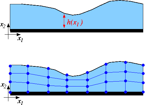
Assume now that we have some discrete representation of the unknown free surface so that is approximated by a function that involves a finite number of discrete unknowns $H_i \ (i=1,...,N_H)$ . In principle, this allows us to represent the unknown boundary by a GeomObject in which the unknowns $H_i \ (i=1,...,N_H)$ play the role of "geometric \c Data", i.e. Data whose values determine the shape of the geometric object. Once the curvilinear boundary is represented by a GeomObject, the update of the nodal positions in the "bulk" mesh could be performed by the Domain / MacroElement - based methods referred to above.

How exactly the unknowns $H_i \ (i=1,...,N_H)$ are determined is irrelevant for the purpose of this discussion ( in free surface flow problems, the relevant equation is the kinematic free-surface condition discussed in another tutorial) – we simply assume that there are some equations that determine their values. The feature we wish to focus on here is that the solution of the problem by Newton's method requires the computation of the derivatives of all discrete residuals with respect to all unknowns in the problem. oomph-lib's Navier-Stokes elements compute the element residual vectors (the residuals of the discretised momentum and continuity equations, evaluated for the current values of the unknowns), and the derivatives of these residuals with respect to the elements' velocity and pressure degrees of freedom. Clearly, the entries in the element's residual vector also depend on the position of the element's constituent nodes, which, in a free-boundary problem, are determined (via the node update function) by the unknowns $H_i \ (i=1,...,N_H)$ that discretise the position of the free surface.

The main purpose of this example is to demonstrate the use (and the creation) of so-called "spine meshes". Such meshes are similar to the MacroElement / Domain - based meshes employed in many previous examples, in that they allow the nodal positions to be updated in response to changes in the shape of their (curvilinear) domain boundaries. The key feature of "spine meshes" is that the node update can be performed on a node-by-node basis – this an important requirement for the efficient solution of free-boundary and fluid-structure interaction problems in which the position of the nodes in the "bulk mesh" is determined by the (unknown) position of the domain boundary. The efficient evaluation of the so-called "shape derivatives" (the derivatives of the residuals of the equations discretised by the elements in the "bulk mesh" with respect to the unknowns that determine the position of the domain boundary)

The idea behind spine-based node updates is illustrated in the sketch below. Assume that the position of the domain boundary is parametrised by a scalar function, so that, for instance, , where may have to be determined as part of the solution (e.g. in free-surface fluids problems – the origin of the "Method of Spines").

Sketch of the Method of Spines.

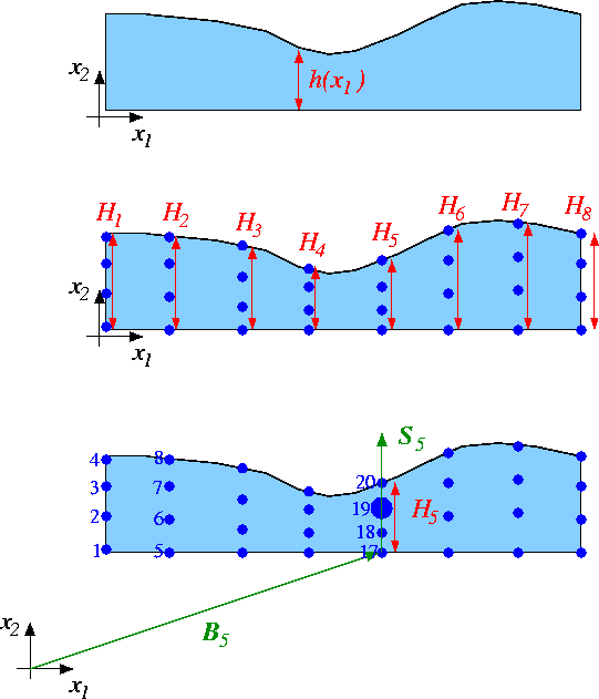
Further, assume that the mesh topology is such that the mesh's $N_{node}$ nodes are distributed along $N_{spine}$ lines that are (topologically) orthogonal to the free boundary. We refer to these lines as the "spines" and denote the "height" of the domain, measured along spine by $H_s \ (s=1,...,N_{spine})$ . We associate each node with a particular spine (so that node is located on spine ) and locate it along a fixed fraction $\omega_j$ along "its" spine. The position of node may therefore be written as

${\bf x}_j = {\bf B}_{s_j} + \omega_j \, H_{s_j} \, {\bf S}_{s_j} \ \ \ \ \ \ \ \ \ \ \ \ \ (1)$

where ${\bf B}_s$ is the vector to the "base" of spine , and ${\bf S}_s$ the unit vector along that spine.

A key feature of this method is that

Determining the nodal positions via the "Method of Spines" equation (1)

Spine-based node updates This document has two main parts:

In Part 1: Flow through a channel of non-uniform width we demonstrate how to use a SpineMesh
In Part 2: How to create a SpineMesh we explain the general "philosophy" behind spine-based node-updates and demonstrate their implementation.

Part 1: Flow through a channel of non-uniform width

The example problem

We shall illustrate the use of SpineMeshes by considering the problem of steady 2D flow through a channel of non-uniform width.

The steady 2D Navier-Stokes equations in a channel of non-uniform width.

Solve

$Re \ u_j\frac{\partial u_i}{\partial x_j} = - \frac{\partial p}{\partial x_i} + \frac{\partial }{\partial x_j} \left( \frac{\partial u_i}{\partial x_j} + \frac{\partial u_j}{\partial x_i} \right),$

and

$\frac{\partial u_i}{\partial x_i} = 0,$

in the region $D = \left\{(x_1,x_2) \ \bigg| \ x_1 \in [0,L], x_2 \in [0,h(x_1)] \right\}$ , where

$h(x_1) = \left\{ \begin{array}{cl} H & 0 \leq x_1 \leq L_1 \\ H + A\sin\left(\frac{x_1-L_1}{L_2-L_1}\right) & L_1 \leq x_1 \leq L_2 \\ H & L_2 \leq x_1 \leq L \end{array} \right.$

shown in this sketch

Sketch of the problem.

subject to the no-slip Dirichlet boundary conditions on the top and bottom rigid walls

$\left. \mathbf{u}\right|_{\partial D_{wall}}=(0,0),$

parallel, parabolic inflow on the left inflow boundary, $\partial D_{inflow} = \{ (x_1,x_2) \ | \ x_1=0 \}$ ,

$\left. \mathbf{u}\right|_{\partial D_{inflow}} =\left(x_2\left(H-x_2\right),0\right),$

and axially traction-free, parallel outflow on the outflow boundary, $\partial D_{outflow} = \{ (x_1,x_2) \ | \ x_1=L \}$ ,

$\left. u_2\right|_{\partial D_{outflow}}=0.$

Results

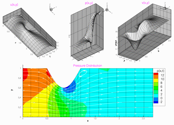
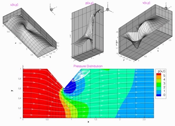
The figures below show the results (carpet plots of the two velocity components and the pressure, and a contour plot of the pressure distribution with superimposed streamlines), obtained from computations with Taylor-Hood and Crouzeix-Raviart elements for a channel of length , height , with deflection amplitude , and a Reynolds number of .

Plot of results computed with 2D Taylor-Hood elements.

Plot of results computed with 2D Crouzeix-Raviart elements.

Global parameters

The Reynolds number is the only parameter in this problem. As usual, we define and initialise it in a namespace:

//==start_of_namespace===================================================
/// Namespace for physical parameters
//=======================================================================
namespace Global_Physical_Variables
{
 
 /// Reynolds number
 double Re=100;
 
} // end_of_namespace

The driver code

We start by creating a DocInfo object to define the output directory.

//==start_of_main======================================================
/// Driver for channel flow problem with spine mesh.
//=====================================================================
int main()
{
 
 // Set output directory
 DocInfo doc_info;
 doc_info.set_directory("RESLT");
 doc_info.number()=0;

When using spines, we must use elements augmented by the SpineElement<ELEMENT> class. This class, adds the functionality to be updated using the method of spines (i.e storing a vector of pointers to the spines and allocating equations numbers associated with the spines degrees of freedom). We build the problem using SpineElement<TayloorHoodElement<2>>.

We now build and solve the problem with Spine-Taylor-Hood elements, then repeat for Spine-Crouzeix-Raviart elements.

 // Solve problem with Taylor Hood elements
 //---------------------------------------
 {
  //Build problem
  ChannelSpineFlowProblem<SpineElement<QTaylorHoodElement<2> > >
   problem;
  
  // Solve the problem with automatic adaptation
  problem.newton_solve();
  
  //Output solution
  problem.doc_solution(doc_info);
  // Step number
  doc_info.number()++;
 
 } // end of Taylor Hood elements
 
 
 // Solve problem with Crouzeix Raviart elements
 //--------------------------------------------
 {
  // Build problem
  ChannelSpineFlowProblem<SpineElement<QCrouzeixRaviartElement<2> > >
   problem;
  
  // Solve the problem with automatic adaptation
  problem.newton_solve();
  
  //Output solution
  problem.doc_solution(doc_info);
  // Step number
  doc_info.number()++;
  
 } // end of Crouzeix Raviart elements
      
 
     
} // end_of_main

The problem class

The problem class for this example is very similar to our previous steady Navier-Stokes examples . We store the height of the channel as private data, this is because we need it to set the inflow boundary condition.

//==start_of_problem_class============================================
/// Channel flow through a non-uniform channel whose geometry is defined 
/// by a spine mesh.
//====================================================================
template<class ELEMENT>
class ChannelSpineFlowProblem : public Problem
{
 
public:
 
 /// Constructor
 ChannelSpineFlowProblem();
 
 /// Destructor: (empty)
 ~ChannelSpineFlowProblem(){}
 
 /// Update the problem specs before solve. 
 /// Set velocity boundary conditions just to be on the safe side...
 void actions_before_newton_solve()
  { 
   // Update the mesh
   mesh_pt()->node_update();
 
  } // end_of_actions_before_newton_solve
 
 
 /// Update the after solve (empty)
 void actions_after_newton_solve(){}
 
 /// Doc the solution
 void doc_solution(DocInfo& doc_info);
 
private:
 
 /// Width of channel
 double Ly;
 
 
}; // end_of_problem_class

Note that the absence of boundary conditions on the right boundary (1), causes a zero traction condition to be applied there. This implies that we should not fix a pressure degree of freedom.

The problem constructor

We begin by setting all the mesh parameters, and building it.

//==start_of_constructor==================================================
/// Constructor for ChannelSpineFlow problem 
//========================================================================
template<class ELEMENT>
ChannelSpineFlowProblem<ELEMENT>::ChannelSpineFlowProblem()
{ 
 
 // Setup mesh
 
 // # of elements in x-direction in left region 
 unsigned Nx0=3;
 // # of elements in x-direction in centre region
 unsigned Nx1=12;
 // # of elements in x-direction in right region
 unsigned Nx2=8;
 
 // # of elements in y-direction
 unsigned Ny=10;
 
 // Domain length in x-direction in left region
 double Lx0=0.5;
 // Domain length in x-direction in centre region
 double Lx1=0.7;
 // Domain length in x-direction in right region
 double Lx2=1.5;
 
 // Domain length in y-direction
 Ly=1.0;
 
 // Build geometric object that represents the sinusoidal bump on
 // the upper wall:
 
 // 40% indendentation
 double amplitude_upper = -0.4*Ly;
 // Minimum and maximum coordinates of bump
 double zeta_min=Lx0;
 double zeta_max=Lx0+Lx1;
 GeomObject* UpperWall = 
  new SinusoidalWall(Ly,amplitude_upper,zeta_min,zeta_max);
 
 // Build and assign mesh -- pass pointer to geometric object
 // that represents the sinusoidal bump on the upper wall
 Problem::mesh_pt() = new ChannelSpineMesh<ELEMENT>(Nx0,Nx1,Nx2,Ny,
                                                    Lx0,Lx1,Lx2,Ly,
                                                    UpperWall);

We then pin the velocities on the left, top and bottom boundaries (3,2 and 0).

 
 
 // Set the boundary conditions for this problem: All nodes are
 // free by default -- just pin the ones that have Dirichlet conditions
 // here: All boundaries are Dirichlet boundaries, except on boundary 1
 unsigned num_bound = mesh_pt()->nboundary();
 for(unsigned ibound=0;ibound<num_bound;ibound++)
  {
   unsigned num_nod= mesh_pt()->nboundary_node(ibound);
   for (unsigned inod=0;inod<num_nod;inod++)
    {
     if (ibound!=1)
      {
       // Loop over values (u and v velocities)
       for (unsigned i=0;i<2;i++)
        {
         mesh_pt()->boundary_node_pt(ibound,inod)->pin(i); 
        }
      }
     else
      {
       // Parallel outflow ==> no-slip
       mesh_pt()->boundary_node_pt(ibound,inod)->pin(1); 
      }
    }
  } // end loop over boundaries

Finally, we pass a pointer to the Reynolds number to each element and assign the equation numbers.

 
 
 // No slip on stationary upper and lower walls (boundaries 0 and 2) 
 // and parallel outflow (boundary 1) 
 for (unsigned ibound=0;ibound<num_bound-1;ibound++)
  {
   unsigned num_nod= mesh_pt()->nboundary_node(ibound);
   for (unsigned inod=0;inod<num_nod;inod++)
    {
     if (ibound!=1)
      {
       for (unsigned i=0;i<2;i++)
        {
         mesh_pt()->boundary_node_pt(ibound,inod)->set_value(i,0.0);
        }
      }
     else
      {
       mesh_pt()->boundary_node_pt(ibound,inod)->set_value(1,0.0);
      }
    }
  }
 
 
 // Setup parabolic inflow along boundary 3:
 unsigned ibound=3; 
 unsigned num_nod= mesh_pt()->nboundary_node(ibound);
 for (unsigned inod=0;inod<num_nod;inod++)
  {
   double y=mesh_pt()->boundary_node_pt(ibound,inod)->x(1);
   // Parallel, parabolic inflow
   mesh_pt()->boundary_node_pt(ibound,inod)->set_value(0,y*(Ly-y));
   mesh_pt()->boundary_node_pt(ibound,inod)->set_value(1,0.0);
  }
 
 // Find number of elements in mesh
 unsigned n_element = mesh_pt()->nelement();
 
 // Loop over the elements to set up element-specific 
 // things that cannot be handled by constructor: Pass 
 // pointer to Reynolds number
 for(unsigned e=0;e<n_element;e++)
  {
   // Upcast from GeneralisedElement to the present element
   ELEMENT* el_pt = dynamic_cast<ELEMENT*>(mesh_pt()->element_pt(e));
   //Set the Reynolds number
   el_pt->re_pt() = &Global_Physical_Variables::Re;
  } 
 
 // Setup equation numbering scheme
 cout <<"Number of equations: " << assign_eqn_numbers() << std::endl; 
 
} // end_of_constructor

Part 2: How to create a SpineMesh

Spine-based meshes have their origin in free-surface fluid-mechanics problems where they were first (?) introduced by Kistler & Scriven in their paper

Kistler, S.F. & Scriven, L.E. Coating Flows.'' In: Computational Analysis of Polymer Processing,'' Pearson, J.R.A. & Richardson, S.M. (eds.); Applied Science Publishers, London (1983).

oomph-lib's SpineMeshes provide a generalisation of their node-update techniques.

In the past when solving a problem in a domain with curved boundaries, we have made a specific Mesh for the domain, and use a geometric object to define its curved wall(s).

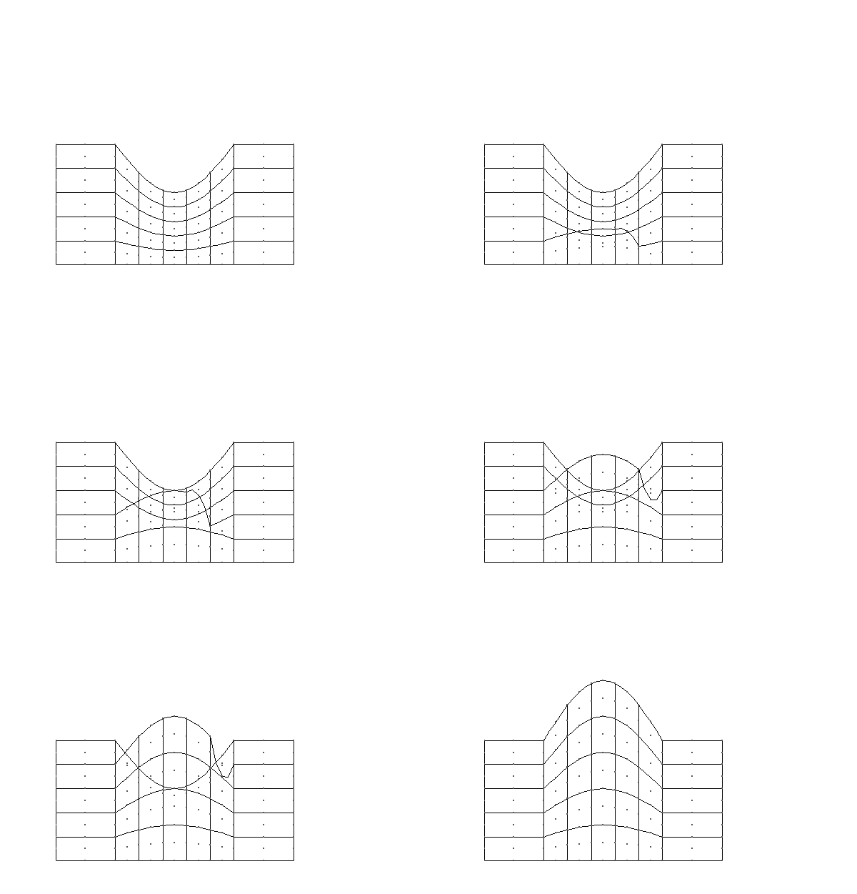
Diagram of a ChannelSpineMesh, going through the process of updating its central nodes, where the heights have been changed.

To generalise this approach oomph-lib makes use of spines.

A Spine is most easily visualised a line of a certain height, in one coordinate direction.
A SpineNode is a Node located at a certain fraction along a Spine.
A SpineMesh is a Mesh which will update using spines.
A SpineElement<ELEMENT> takes a "normal" element and adds the functionality to work with spines.

The creation of a SpineMesh is discussed in detail below Making a SpineMesh. While the picture above demonstrates the ability of SpineNode to individually update using the function spine_node_update(spine_node_pt).

Making a SpineMesh

In this example we use a SpineMesh to model the domain. This mesh constitutes three regions: left (0), centre (1) and right (2), the left and right regions have a constant height, while in the centre region the height varies. These heights are defined by two geometric objects, a straight line and a deflected line respectively. We will discuss the necessary steps taken to create this mesh (the complete documentation for this specific mesh can be found here ).

To begin, we create a new class templated by a element and inheriting from RectangularQuadMesh<ELEMENT> and SpineMesh. The latter adds the functionality needed for using Spines.

template<class ELEMENT>

class ChannelSpineMesh : public RectangularQuadMesh<ELEMENT>, public SpineMesh

All SpineMeshs must include a function spine_node_update(SpineNode* spine_node_pt), this will describe the operations performed when updating every SpineNode in the mesh. First we find the SpineNodes fraction along the spine.

    virtual void spine_node_update(SpineNode* spine_node_pt)
    {
      // Get spine node's fraction along the spine
      double W = spine_node_pt->fraction();

We then get the local coordinate on the geometric object that defines the upper wall.

 
      // Get local coordinates
      Vector<double> s_wall(1);
      s_wall[0] = spine_node_pt->spine_pt()->geom_parameter(0);

Finally we use the use the local coordinate to get the position of the geometric object and set the first coordinate value of the node.

 
      // Get position vector to wall
      Vector<double> position(2);
      spine_node_pt->spine_pt()->geom_object_pt(0)->position(s_wall, position);
 
      // Set the value of y
      spine_node_pt->x(1) = this->Ymin + W * position[1];
    }

We store the number of elements in the x direction in each region, the number of elements in the y direction, the lengths of each region and the height of the uniform boundary, as well as pointers to the two geometric objects.

    /// Number of elements in the left region
    unsigned Nx0;
 
    /// Number of elements in the centre region
    unsigned Nx1;
 
    /// Number of elements in the right region
    unsigned Nx2;
 
    /// Length of left region
    double Lx0;
 
    /// Length of centre region
    double Lx1;
 
    /// Length of right region
    double Lx2;
 
    /// Number of spines in left region
    unsigned Nleft_spine;
 
    /// Number of spines in centre region
    unsigned Ncentre_spine;
 
    /// Number of spines in right region
    unsigned Nright_spine;
 
    /// GeomObject for upper wall
    GeomObject* Wall_pt;
 
    /// GeomObject for the straight upper wall
    GeomObject* Straight_wall_pt;

All these details are passed to the constructor, except for the pointer to the geometric object for the uniform wall. The constructor calls the empty constructor for RectangularQuadMesh<ELEMENT>, copies these values to their storage in the mesh.

  template<class ELEMENT>
  ChannelSpineMesh<ELEMENT>::ChannelSpineMesh(const unsigned& nx0,
                                              const unsigned& nx1,
                                              const unsigned& nx2,
                                              const unsigned& ny,
                                              const double& lx0,
                                              const double& lx1,
                                              const double& lx2,
                                              const double& h,
                                              GeomObject* wall_pt,
                                              TimeStepper* time_stepper_pt)
    : RectangularQuadMesh<ELEMENT>(nx0 + nx1 + nx2,
                                   ny,
                                   0.0,
                                   lx0 + lx1 + lx2,
                                   0.0,
                                   h,
                                   false,
                                   false,
                                   time_stepper_pt),
      Nx0(nx0),
      Nx1(nx1),
      Nx2(nx2),
      Lx0(lx0),
      Lx1(lx1),
      Lx2(lx2),
      Wall_pt(wall_pt)

We then assign all the parameters for the RectangularQuadMesh<ELEMENT>, create the geometric object for the uniform wall and call the function build_channel_spine_mesh(...)

  {
    // Mesh can only be built with 2D Qelements.
    MeshChecker::assert_geometric_element<QElementGeometricBase, ELEMENT>(2);
 
    // Mesh can only be built with spine elements
    MeshChecker::assert_geometric_element<SpineFiniteElement, ELEMENT>(2);
 
    // We've called the "generic" constructor for the RectangularQuadMesh
    // which doesn't do much...
 
    // Build the straight line object
    Straight_wall_pt = new StraightLine(h);
 
    // Now build the mesh:
    build_channel_spine_mesh(time_stepper_pt);
  }

When we call the function build_channel_spine_mesh(...), it calls its counterpart in the RectangularQuadMesh<ELEMENT>, then store the numbers of elements in each direction in each region (and all at once).

  void ChannelSpineMesh<ELEMENT>::build_channel_spine_mesh(
    TimeStepper* time_stepper_pt)
  {
    // Build the underlying quad mesh:
    RectangularQuadMesh<ELEMENT>::build_mesh(time_stepper_pt);
 
    // Read out the number of elements in the x-direction and y-direction
    // and in each of the left, centre and right regions
    unsigned n_x = this->Nx;
    unsigned n_y = this->Ny;
    unsigned n_x0 = this->Nx0;
    unsigned n_x1 = this->Nx1;
    unsigned n_x2 = this->Nx2;

We then allocate memory for the elements and spines in each region in each region.

 
    // Set up the pointers to elements in the left region
    unsigned nleft = n_x0 * n_y;
    ;
    Left_element_pt.reserve(nleft);
    unsigned ncentre = n_x1 * n_y;
    ;
    Centre_element_pt.reserve(ncentre);
    unsigned nright = n_x2 * n_y;
    ;
    Right_element_pt.reserve(nright);
    for (unsigned irow = 0; irow < n_y; irow++)
    {
      for (unsigned e = 0; e < n_x0; e++)
      {
        Left_element_pt.push_back(this->finite_element_pt(irow * n_x + e));
      }
      for (unsigned e = 0; e < n_x1; e++)
      {
        Centre_element_pt.push_back(
          this->finite_element_pt(irow * n_x + (n_x0 + e)));
      }
      for (unsigned e = 0; e < n_x2; e++)
      {
        Right_element_pt.push_back(
          this->finite_element_pt(irow * n_x + (n_x0 + n_x1 + e)));
      }
    }
 
#ifdef PARANOID
    // Check that we have the correct number of elements
    if (nelement() != nleft + ncentre + nright)
    {
      throw OomphLibError("Incorrect number of element pointers!",
                          OOMPH_CURRENT_FUNCTION,
                          OOMPH_EXCEPTION_LOCATION);
    }
#endif
 
    // Allocate memory for the spines and fractions along spines
    //---------------------------------------------------------
 
    // Read out number of linear points in the element
    unsigned n_p = dynamic_cast<ELEMENT*>(finite_element_pt(0))->nnode_1d();
 
    unsigned nspine;
    // Allocate store for the spines:
    if (this->Xperiodic)
    {
      nspine = (n_p - 1) * n_x;
      Spine_pt.reserve(nspine);
      // Number of spines in each region
      // NOTE that boundary spines are in both regions
      Nleft_spine = (n_p - 1) * n_x0 + 1;
      Ncentre_spine = (n_p - 1) * n_x1 + 1;
      Nright_spine = (n_p - 1) * n_x2;
    }
    else
    {
      nspine = (n_p - 1) * n_x + 1;
      Spine_pt.reserve(nspine);
      // Number of spines in each region
      // NOTE that boundary spines are in both regions
      Nleft_spine = (n_p - 1) * n_x0 + 1;
      Ncentre_spine = (n_p - 1) * n_x1 + 1;
      Nright_spine = (n_p - 1) * n_x2 + 1;
    }
 
    // end Allocating memory

Now we allocate storage for the parameters used to build the spines.

 
 
    // set up the vectors of geometric data & objects for building spines
    Vector<double> r_wall(2), zeta(1), s_wall(1);
    GeomObject* geometric_object_pt = 0;
 
    // LEFT REGION
    // ===========
 
    // SPINES IN LEFT REGION
    // ---------------------
 
    // Set up zeta increments
    double zeta_lo = 0.0;
    double dzeta = Lx0 / n_x0;
 
    // Initialise number of elements in previous regions:
    unsigned n_prev_elements = 0;

Now we create the first Spine with unit length, pin the height (since it is not a degree of freedom in this mesh) and push the spine back onto the Spine_pt.

 
 
    // FIRST SPINE
    //-----------
 
    // Element 0
    // Node 0
    // Assign the new spine with unit length
    Spine* new_spine_pt = new Spine(1.0);
    new_spine_pt->spine_height_pt()->pin(0);
    Spine_pt.push_back(new_spine_pt);

We then set the spine_pt() of the first node to the Spine we just created, assign the nodes fraction() to zero and define the node as part of this mesh.

 
    // Get pointer to node
    SpineNode* nod_pt = element_node_pt(0, 0);
    // Set the pointer to the spine
    nod_pt->spine_pt() = new_spine_pt;
    // Set the fraction
    nod_pt->fraction() = 0.0;
    // Pointer to the mesh that implements the update fct
    nod_pt->spine_mesh_pt() = this;

We then mark the node as part of the left (0) region.

// Set update fct id

nod_pt->node_update_fct_id() = 0;

When we built the Spine, we set its height to 1.0. We now need to assign its height from the Straight_wall_pt and assign all the information needed to update the mesh to the Spine.

First we set the value of $\zeta$ and get the geometric object and the local coordinate.

 
    // Provide spine with additional storage for wall coordinate
    // and wall geom object:
 
    {
      // Get the Lagrangian coordinate in the Lower Wall
      zeta[0] = 0.0;
      // Get the geometric object and local coordinate
      Straight_wall_pt->locate_zeta(zeta, geometric_object_pt, s_wall);

Then we store these geometric parameters in the Spine.

 
      // The local coordinate is a geometric parameter
      // This needs to be set (rather than added) because the
      // same spine may be visited more than once
      Vector<double> parameters(1, s_wall[0]);
      nod_pt->spine_pt()->set_geom_parameter(parameters);

We then set the height of the Spine according to the geometric object.

 
      // Get position of wall
      Straight_wall_pt->position(s_wall, r_wall);
 
      // Adjust spine height
      nod_pt->spine_pt()->height() = r_wall[1];

Finally we set the Spines' pointer to the geometric object.

 
      // The sub geom object is one (and only) geom object
      // for spine:
      Vector<GeomObject*> geom_object_pt(1);
      geom_object_pt[0] = geometric_object_pt;
 
      // Pass geom object(s) to spine
      nod_pt->spine_pt()->set_geom_object_pt(geom_object_pt);
    }

Now we loop vertically along the spine, adding a pointer to the spine to each element, and assigning the fraction for each node on this spine, define each node as part of this mesh, and mark it as part of the left region.

 
    // Loop vertically along the spine
    // Loop over the elements
    for (unsigned long i = 0; i < n_y; i++)
    {
      // Loop over the vertical nodes, apart from the first
      for (unsigned l1 = 1; l1 < n_p; l1++)
      {
        // Get pointer to node
        SpineNode* nod_pt = element_node_pt(i * n_x, l1 * n_p);
        // Set the pointer to the spine
        nod_pt->spine_pt() = new_spine_pt;
        // Set the fraction
        nod_pt->fraction() =
          (double(i) + double(l1) / double(n_p - 1)) / double(n_y);
        // Pointer to the mesh that implements the update fct
        nod_pt->spine_mesh_pt() = this;
        // Set update fct id
        nod_pt->node_update_fct_id() = 0;
      }
    } // end loop over elements

We then loop over the remaining spines in the left region repeating this process, except that the first spine in each element (except the first) is copied from the last spine in the previous element.

We then repeat this process for the centre and right regions, using the correct geometric objects to define the upper wall, which can be examined in detail here .

Exercises

Investigate what happens when a pressure degree of freedom is fixed.
Try creating a new geometric object, which creates a triangular indentation in the central region of the upper wall as shown.

Plot of the solution to the problem specified in the above exercise computed with 3x3 Taylor-Hood elements and Re=100.

PDF file

A pdf version of this document is available.