In this tutorial we present an example of surface-transport equations in a free-surface Navier–Stokes problem. This is a multi-domain, multi-physics problem because there is a coupling between the equations on the surface and those in the bulk. The coupling from the bulk to the surface transport arises through the surface velocity in the surface transport equation. The coupling from the surface transport to bulk arises in a more subtle manner because the surface concentration affects the surface tension. In this tutorial, we describe how to use the existing framework to create surface transport equations and how to include them in a free-surface problem.

The example problem

The problem to be solved is the evolution of an annular film of fluid on the inside of a solid cylinder in the presence of an insoluble surfactant on the interface: a modification of the classic Rayleigh–Plateau instability. For validation, we reproduce some of the results given in `A 2-D model of Rayleigh instability in capillary tubes — surfactant effects' by D. Campana, J. Di Paolo & F. A. Saita, Int. J. Multiphase Flow, vol 30 , pp 431–454, (2004). Our formulation, however, is different from their approach as described in detail in our free-surface theory document.

The unsteady axisymmetric free-surface Navier–Stokes equations with insoluble surfactant .

Solve

$Re \left[ St \frac{\partial u_r}{\partial t} + u_r \frac{\partial u_r}{\partial r} - \frac{u_\theta^2}{r} + u_z \frac{\partial u_r}{\partial z} \right] = -\frac{\partial p}{\partial r} + \left[ \frac{\partial^2 u_r}{\partial r^2} + \frac{1}{r}\frac{\partial u_r}{\partial r} - \frac{u_r}{r^2} + \frac{\partial^2 u_r}{\partial z^2} \right],$

$Re \left[ St \frac{\partial u_\theta}{\partial t} + u_r \frac{\partial u_\theta}{\partial r} + \frac{u_r u_\theta}{r} + u_z \frac{\partial u_\theta}{\partial z} \right] = + \left[ \frac{\partial^2 u_\theta}{\partial r^2} + \frac{1}{r}\frac{\partial u_\theta}{\partial r} - \frac{u_\theta}{r^2} + \frac{\partial^2 u_\theta}{\partial z^2} \right],$

$Re \left[ St \frac{\partial u_z}{\partial t} + u_r \frac{\partial u_z}{\partial r} + u_z \frac{\partial u_z}{\partial z} \right] = -\frac{\partial p}{\partial z} + \left[ \frac{\partial^2 u_z}{\partial r^2} + \frac{1}{r}\frac{\partial u_z}{\partial r} + \frac{\partial^2 u_z}{\partial z^2} \right],$

and

$\frac{\partial u_r}{\partial r} + \frac{u_r}{r} + \frac{\partial u_z}{\partial z} = 0 \ \ \ \ \ \ \ \ \ \ (1)$

in the bulk fluid.

The governing equations are subject to the no slip boundary conditions

$u_r = u_\theta = u_z = 0 \ \ \ \ \ \ \ \ \ \ (2)$

on the outer solid boundary ( ) and the symmetry boundary conditions

$u_z = u_\theta = 0 \ \ \ \ \ \ \ \ \ \ (3)$

on the bottom ( ) and top ( $z = \pi / \alpha$ ) boundaries.

We denote the position vector to the free surface by $\mathbf{R}$ , which is subject to the kinematic condition

$\left(u_i - St\, \frac{\partial R_i}{\partial t}\right) n_i = 0, \ \ \ \ \ \ \ \ \ \ (4)$

and the dynamic condition

$\tau_{ij}^{[2]}n_j = \tau_{ij}^{[1]}n_j+\frac{1}{Ca}\left (\sigma \kappa n_i + \frac{\partial \sigma}{\partial s} t_{i} \right). \ \ \ \ \ \ \ \ \ \ (5)$

where $\sigma = \sigma^{*} / \sigma_{ref}$ is the dimensionless surface tension relative to a reference value.

An insoluble surfactant of surface concentration $\Gamma^{*}$ is non-dimensionalised with respect to a reference value $\Gamma = \Gamma^{*}/\Gamma_{ref}$ and obeys the surface transport equation

$St \left(\frac{\partial \Gamma}{\partial t} - \dot{\mbox{\boldmath$R$}} \mbox{\boldmath$\cdot$} \mbox{\boldmath$\nabla$}_{\!\!_{S}} \Gamma \right) + \mbox{\boldmath$\nabla$}_{\!\!_{S}} \mbox{\boldmath$\cdot$} \left(\Gamma \mbox{\boldmath$U$}\right) = \frac{1}{Pe_{s}} \mbox{\boldmath$\nabla$}_{\!\!_{S}}\mbox{\boldmath$\cdot$} \mbox{\boldmath$\nabla$}_{\!\!_{S}} \Gamma$

on the interface.

The surface tension is a function of the surfactant concentration $\sigma(\Gamma)$ and a linear equation of state is chosen

$\sigma = 1 - \beta (\Gamma - 1).$

The symmetry boundary conditions on the bottom ( ) and top ( $z = \pi / \alpha$ ) boundaries are

$\frac{\partial \Gamma}{\partial z} = 0.$

Initially, the system is at rest and $\Gamma =1$ . The free surface is moved into the position:

$\mathbf{R} = \left[1.0 - H*(1.0 + \epsilon\cos \left(\alpha z\right) \right] \mbox{\boldmath$e$}_{r}$

where $\epsilon$ is a small parameter and is the undeformed film thickness.

Results

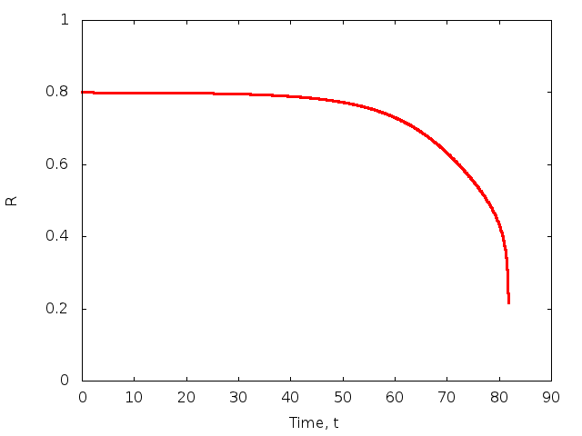
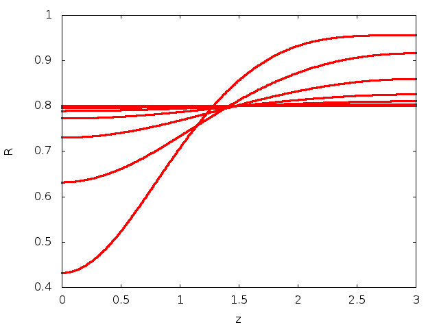
We choose parameters based on those used to compute Figures 8 and 9 in Campana et al; namely , , , $Ca = H^{3}$ , $\alpha = 1.047$ , $\epsilon = 10^{-3}$ , $\beta = 3.6 \times 10^{-3}$ and $Pe_{S} = 4032$ . For these parameters, the system is unstable to the Rayleigh–Plateau instability and evolves towards a state in which the tube is completely occluded by the fluid at one end.

Time trace of the radius of the interface at z=0 showing dramatic collapse near t=80.

Evolution of the interface at times t=0, 10, 20, 30, 40, 50, 60, 70, 80 showing the developing lobe.

Evolution of the surfactant concentration on the interface at times t=0, 10, 20, 30, 40, 50, 60, 70, 80 accumulation in the developing lobe caused by the reduced surface area and advective flow into the lobe.

Global parameters and functions

The global parameters are simply the dimensionless parameters described above.

//==start_of_namespace===================================================
/// Namespace for physical parameters
/// The parameter values are chosen to be those used in Figures 8, 9 
/// in Campana et al.
//=======================================================================
namespace Global_Physical_Variables
{
 
  //Film thickness parameter
 double Film_Thickness = 0.2;
 
 /// Reynolds number
 double Re = 40.0;
 
 /// Womersley number
 double ReSt = Re; // (St = 1)
 
 /// Product of Reynolds number and inverse of Froude number
 double ReInvFr = 0.0; // (Fr = 0)
 
 /// Capillary number
 double Ca = pow(Film_Thickness,3.0);
 
 /// External pressure
 double P_ext = 0.0;
 
 /// Direction of gravity
 Vector<double> G(3);
 
 /// Wavelength of the domain
 double Alpha = 1.047;
 
 /// Free surface cosine deformation parameter
 double Epsilon = 1.0e-3;
 
 /// Surface Elasticity number (weak case)
 double Beta = 3.6e-3;
 
 /// Surface Peclet number
 double Peclet_S = 4032.0;
 
 /// Sufrace Peclet number multiplied by Strouhal number
 double Peclet_St_S = 1.0; 
 
 /// Pvd file -- a wrapper for all the different
 /// vtu output files plus information about continuous time
 /// to facilitate animations in paraview
 ofstream Pvd_file;
 
} // End of namespace

The driver code and problem class

The driver code and problem are very similar to those in the two-dimensional and axisymmetric interface-relaxation problems on which this driver was based. The main difference between this problem and standard free surface problems is that instead of
oomph::SpineAxisymmetricFluidInterfaceElement, we use the custom oomph::SpineAxisymmetricMarangoniSurfactantFluidInterfaceElement. The symmetry boundary conditions for the surface concentration are the natural boundary conditions of our formulation, so we "do nothing" for the additional field at the boundaries.

An additional member function InterfaceProblem::compute_total_mass() is provided as a check on the implementation of the the surface transport equations. The surfactant cannot be removed from the surface, so its mass must be conserved. The function simply loops over the interface elements and sums their contribution to the total mass.

 /// Compute the total mass of the insoluble surfactant
 double compute_total_mass()
  {
   //Initialise to zero
   double mass = 0.0;
   
   // Determine number of 1D interface elements in mesh
   const unsigned n_interface_element = Interface_mesh_pt->nelement();
   
   // Loop over the interface elements
   for(unsigned e=0;e<n_interface_element;e++)
    {
     // Upcast from GeneralisedElement to the present element
     SpineAxisymmetricMarangoniSurfactantFluidInterfaceElement<ELEMENT>* el_pt = 
      dynamic_cast<SpineAxisymmetricMarangoniSurfactantFluidInterfaceElement<ELEMENT>*>
      (Interface_mesh_pt->element_pt(e));
     //Add contribution from each element
     mass += el_pt->integrate_c();
    }
   return mass;
  } // End of compute_total_mass

The SpineAxisymmetricMarangoniSurfactantFluidInterfaceElement class

This class is implemented in our driver code and inherits directly from oomph::SpineAxisymmetricFluidInterfaceElement. The class provides storage for the required additional dimensionless groups and the nodal index where the surface concentration will be stored.

/// Spine-based Marangoni surface tension elements that add
/// a linear dependence on concentration
/// of a surface chemical to the surface tension, 
/// which decreases with increasing concentration.
/// The non-dimensionalisation is the same as Campana et al (2004)
/// but we may wish to revisit this.
//=================================================================
template<class ELEMENT>
class SpineAxisymmetricMarangoniSurfactantFluidInterfaceElement : 
  public SpineAxisymmetricFluidInterfaceElement<ELEMENT>
{
private:
 /// Pointer to an Elasticity number
  double *Beta_pt;
 
 /// Pointer to Surface Peclet number
  double *Peclet_S_pt;
 
 /// Pointer to the surface Peclect Strouhal number
  double *Peclet_Strouhal_S_pt;
 
 /// Index at which the surfactant concentration is stored at the
 /// nodes
 unsigned C_index;

Most of the functionality is already provided by the underlying FluidInterfaceElement and we need simply to overload a few functions. The constructor sets default values for the physical constants and adds the additional data value to nodes on the surface.

 /// Constructor that passes the bulk element and face index down
 /// to the underlying
  SpineAxisymmetricMarangoniSurfactantFluidInterfaceElement(FiniteElement* const &element_pt, const int &face_index) : SpineAxisymmetricFluidInterfaceElement<ELEMENT>
                                                                                                                       (element_pt,face_index)
  {
   //Initialise the values
   Beta_pt = &Default_Physical_Constant_Value;
   Peclet_S_pt = &Default_Physical_Constant_Value;
   Peclet_Strouhal_S_pt = &Default_Physical_Constant_Value;
 
   //Add the additional surfactant terms to these surface elements
   
   //Read out the number of nodes on the face
   //For some reason I need to specify the this pointer here(!)
   unsigned n_node_face = this->nnode();
   //Set the additional data values in the face
   //There is one additional values at each node --- the lagrange multiplier
   Vector<unsigned> additional_data_values(n_node_face);
   for(unsigned i=0;i<n_node_face;i++) additional_data_values[i] = 1;
   //Resize the data arrays accordingly 
   this->resize_nodes(additional_data_values);
 
   //The C_index is the new final value
   //Minor HACK HERE
   C_index = this->node_pt(0)->nvalue()-1;
}

The function FluidInterfaceElement::sigma() is overloaded using the equation of state defined in the problem specification

 double sigma(const Vector<double> &s)
  {
   //Find the number of shape functions
   const unsigned n_node = this->nnode();
   //Now get the shape fuctions at the local coordinate
   Shape psi(n_node);
   this->shape(s,psi);
   
   //Now interpolate the surfactant concentration
   double C=0.0;
   for(unsigned l=0;l<n_node;l++)
    {
     C += this->nodal_value(l,C_index)*psi(l);
    }
   
   //Get the Elasticity number
   double Beta = this->beta();
   //Return the variable surface tension
   return (1.0 - Beta*(C-1.0));
  } // End of sigma

The majority of the work is performed in

  void add_additional_residual_contributions_interface(Vector<double> &residuals, DenseMatrix<double> &jacobian,
                                                       const unsigned &flag,const Shape &psif, const DShape &dpsifds,
                                                       const DShape &dpsifdS, const DShape &dpsifdS_div,
                                                       const Vector<double> &s,
                                                       const Vector<double> &interpolated_x, const Vector<double> &interpolated_n, 
                                                       const double &W,const double &J)
  {

which provides the additional surface transport equations. In the example code two formulations of the surface transport equations are provided the one used by Campana et al in which the curvature is computed explicitly and the formulation derived in our free-surface theory, in which the curvature is not required. The version used is determined by an internal boolean

   //Flag to control whether the Campana formulation (false) 
   // or our own (true) is used
   bool Integrated_curvature = true;

The remainder of the function adds the residuals associated with the surfactant transport equations which are described in the free-surface theory. Note that an additional term arises due to the azimuthal curvature compared to the standard one-dimensional surface.

The function fill_in_contribution_to_jacobian(...) is also overloaded to that the effect of surfactant concentration on the bulk equations is computed by finite differences. This could be modified in the future so that the appropriate derivative terms are included in add_additional_residual_contributions_interface(...).

Finally the elements contain a function

 double integrate_c() const
  {
   //Find out how many nodes there are
   unsigned n_node = this->nnode();
   
   //Set up memeory for the shape functions
   Shape psif(n_node);
   DShape dpsifds(n_node,1);
 
   //Set the value of n_intpt
   unsigned n_intpt = this->integral_pt()->nweight();
   
   //Storage for the local coordinate
   Vector<double> s(1);
 
   //Storage for the total mass
   double mass = 0.0;
   
   //Loop over the integration points
   for(unsigned ipt=0;ipt<n_intpt;ipt++)
    {
     //Get the local coordinate at the integration point
     s[0] = this->integral_pt()->knot(ipt,0);
     
     //Get the integral weight
     double W = this->integral_pt()->weight(ipt);
     
     //Call the derivatives of the shape function
     this->dshape_local_at_knot(ipt,psif,dpsifds);
     
     //Define and zero the tangent Vectors and local velocities
     Vector<double> interpolated_x(2,0.0);
     Vector<double> interpolated_t(2,0.0);
     double interpolated_c = 0.0;
     
     
     //Loop over the shape functions to compute concentration and tangent
     for(unsigned l=0;l<n_node;l++)
      {
       interpolated_c += this->nodal_value(l,C_index)*psif(l);
       //Calculate the tangent vector
       for(unsigned i=0;i<2;i++)
        {
         interpolated_x[i] += this->nodal_position(l,i)*psif(l);
         interpolated_t[i] += this->nodal_position(l,i)*dpsifds(l,0);
        }
      }
     
     //The first positional coordinate is the radial coordinate
     double r = interpolated_x[0];
 
   //Calculate the length of the tangent Vector
   double tlength = interpolated_t[0]*interpolated_t[0] + 
    interpolated_t[1]*interpolated_t[1];
   
   //Set the Jacobian of the line element
   double J = sqrt(tlength);
 
   mass += interpolated_c*r*W*J;
    }
   return mass;
  }
 
};
 
 
//Define the default physical value to be one
template<class ELEMENT>
double SpineAxisymmetricMarangoniSurfactantFluidInterfaceElement<ELEMENT>::Default_Physical_Constant_Value = 1.0;
 
}
 
 
namespace oomph
{
 
//======================================================================
/// Inherit from the standard Horizontal single-layer SpineMesh
/// and modify the spine_node_update() function so that it is appropriate
/// for an annular film, rather than a fluid fibre.
//======================================================================
template <class ELEMENT>
class MyHorizontalSingleLayerSpineMesh : 
  public HorizontalSingleLayerSpineMesh<ELEMENT>
{
 
public:
 
 /// Constructor: Pass number of elements in x-direction, number of
 /// elements in y-direction, radial extent, axial length , and pointer 
 /// to timestepper (defaults to Steady timestepper)
 MyHorizontalSingleLayerSpineMesh(const unsigned &nx, 

that computes the integral of the concentration over the elemental surface, representing the total mass of surfactant within the element.

Exercises

Investigate the difference between the solutions for the two formulations of the surfactant transport equations. Which conserves mass more accurately?
Investigate the influence of variations in $\beta$ and try to reproduce the results found by Campana et al.
Look at the three-dimensional (non-axisymmetric) version of the code found in the same directory. Confirm that the same results are produced. Is the instability stable to non-axisymmetric perturbations? Use the code to investigate what happens if you make the cross-sectional boundary slightly elliptical rather than circular?

Source files for this tutorial

The source files for this tutorial are located in the directory:

demo_drivers/multi_physics/rayleigh_instability_surfactant

which contains refineable and non-refineable multi-domain versions of the Boussinesq convection problem.
The full driver code for the problem described in this tutorial is:

demo_drivers/multi_physics/rayleigh_instability_surfactant/rayleigh_instability_insoluble_surfactant.cc
The corresponding driver code for the non-refineable version of the problem is:

demo_drivers/multi_physics/boussinesq_convection/multi_domain_boussinesq_convection.cc

PDF file

A pdf version of this document is available.