In this document, we demonstrate how to solve a 1D eigenproblem (eigenvalues of the shifted 1D Laplace operator in a bounded domain) by creating custom elements. The tutorial is related to the harmonic eigenproblem , which you should read first. The fundamental difference in this case, is that we treat the eigenproblem as two coupled first-order equations which ensures that many of the eigenvalues are complex.

One-dimensional model eigenvalue problem with complex eigenvalues Solve

$\frac{\partial u}{\partial x} = (\lambda - \mu) w, \quad \frac{\partial w}{\partial x} = \lambda u \ \ \ \ \ \ \ \ \ \ (1)$

in the domain $D =\left\{ x_1 \in [0,1] \right\}$ , with homogeneous Dirichlet boundary conditions

$\left. u\right|_{\partial D}=0. \ \ \ \ \ \ \ \ \ \ (2)$

We shall treat $\lambda$ as an eigenvalue (unknown), but the other parameter $\mu$ is a shift, which is used to modify the spectrum of the operator. The two first-order equations may be combined into a single second-order equation

$\frac{\partial^{2} u}{\partial x^{2}} = (\lambda - \mu) \frac{\partial w}{\partial x} = (\lambda - \mu) \lambda u \quad \Rightarrow\quad \frac{\partial^{2} u}{\partial x^{2}} + (\mu - \lambda) \lambda u = 0,$

which is exactly the same equation as the harmonic eigenproblem , but with a redefinition of the eigenvalues. Hence, the exact solutions are given by the countably infinite set:

$u_{n} = \sin (\Lambda_{n} x_{1}), \ \ \ \ \ \ \ \Lambda_{n} = n \pi = \sqrt{\lambda_{n}(\mu - \lambda_{n})},$

which yields

$\lambda_{n} = \frac{\mu}{2} \pm \sqrt{\mu^{2}/4 - n^{2}\pi^{2}}. \ \ \ \ \ \ \ \ \ \ (3)$

If the shift $\mu = 0$ , then the eigenvalues are all imaginary and consist of the complex conjugate pairs given by $\lambda{n} = \pm n \pi\, \mbox{i}$ .

If $\mu^{2}/4 > \pi^{2}$ $\Rightarrow$ $\mu > 2\pi$ , then the first complex conjugate pair of imaginary eigenvalues becomes two distinct real eigenvalues because the term under the square root in (3) becomes positive. As $\mu$ increases further subsequent complex eigenvalues merge to be real. Thus, we can control the spectrum by modifying the parameter $\mu$ .

We now provide a detailed discussion of the driver code complex_harmonic.cc which solves the problem for the first four eigenvalues, when $\mu = 6.5 > 2\pi.$

Overview of the theory

Weak formulation of the problem

If we wish to solve the problem (1) using finite elements, we simply multiply each equation by a test function, but do not integrate by parts. We shall use the same test functions for each variable and thus our governing equations become

$\int_{D} \frac{\partial u}{\partial x} \phi^{(test)} \,\mbox{d} x = (\lambda -\mu) \int_{D} w\, \phi^{(test)}\,\mbox{d} x, \quad\quad \int_{D} \frac{\partial w}{\partial x} \phi^{(test)} \,\mbox{d} x = \lambda \int_{D} u\, \phi^{(test)}\,\mbox{d} x, \quad$

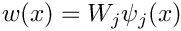If we expand $u(x) = U_{j} \psi_{j}(x)$ and $w(x) = W_{j} \psi_{j}(x)$ in terms of known basis functions $\psi_{j}$ and use the same basis functions as our test functions (Galerkin method), then the weak form becomes

$\int_{D} \frac{\partial \psi_{j}}{\partial x} \psi_{i} \,\mbox{d} x U_{j} = (\lambda - \mu) \int_{D} \psi_{i} \psi_{j}\,\mbox{d} x W_{j},\quad\quad \int_{D} \frac{\partial \psi_{j}}{\partial x} \psi_{i} \,\mbox{d} x W_{j} = \lambda \int_{D} \psi_{i} \psi_{j}\,\mbox{d} x U_{j}.$

Thus, in order to form the discrete eigenproblem 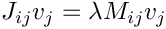$J_{ij} v_{j} = \lambda M_{ij} v_{j}$ , we choose to order the unknowns in the form $v = [ U | W ]^{T}$ , leading to the block Jacobian and mass matrices

$J = \left[\begin{array}{c|c} 0 & A \\\hline A & \mu B \end{array}\right],\quad M = \left[\begin{array}{c|c} B & 0 \\\hline 0 & B \end{array}\right],$

where

$A_{ij} = \int_{D} \frac{\partial \psi_{j}}{\partial x} \psi_{i} \,\mbox{d} x , \quad\quad B_{ij} = \int_{D} \psi_{i} \psi_{j}\,\mbox{d} x.$

Implementation

The implementation closely follows that in the harmonic eigenproblem , and so we shall concentrate on the differences from that problem.

Creating the elements

For generality, we implement the mathematics to assemble contributions to the Jacobian and mass matrices defined above in the class ComplexHarmonicEquations that inherits from FiniteElement.

/// A class for all elements that solve the eigenvalue problem
/// \f[ 
/// \frac{\partial w}{\partial x}  = \lambda u
/// \f] 
/// \f[
/// \frac{\partial u}{\partial x} = (\lambda - \mu) w
/// \f]
/// This class  contains the generic maths. Shape functions, geometric
/// mapping etc. must get implemented in derived class.
//================================================================
class ComplexHarmonicEquations : public virtual FiniteElement
{
 
public:
 /// Empty Constructor
 ComplexHarmonicEquations() {}

The unknowns that represent the discretised eigenfunction are assumed to be stored at the nodes, but there are now two unknowns: is assumed to be the first and is the second.

 /// Access function: First eigenfunction value at local node n
 /// Note that solving the eigenproblem does not assign values
 /// to this storage space. It is used for output purposes only.
 virtual inline double u(const unsigned& n) const 
  {return nodal_value(n,0);}
 
 /// Second eigenfunction value at local node n
 virtual inline double w(const unsigned& n) const 
  {return nodal_value(n,1);}

As before, the key function is fill_in_contribution_to_jacobian_and_mass_matrix which implements the calculation of the equations.

 void fill_in_contribution_to_jacobian_and_mass_matrix(
  Vector<double> &residuals,
  DenseMatrix<double> &jacobian, DenseMatrix<double> &mass_matrix)
  {
   //Find out how many nodes there are
   unsigned n_node = nnode();
   
   //Set up memory for the shape functions and their derivatives
   Shape psi(n_node);
   DShape dpsidx(n_node,1);
 
   //Set the number of integration points
   unsigned n_intpt = integral_pt()->nweight();
   
   //Integers to store the local equation and unknown numbers
   int local_eqn=0, local_unknown=0;
   
   //Loop over the integration points
   for(unsigned ipt=0;ipt<n_intpt;ipt++)
    {
     //Get the integral weight
     double w = integral_pt()->weight(ipt);
     
     //Call the derivatives of the shape and test functions
     double J = dshape_eulerian_at_knot(ipt,psi,dpsidx);
     
     //Premultiply the weights and the Jacobian
     double W = w*J;
 
     //Assemble the contributions to the mass matrix
     //Loop over the test functions
     for(unsigned l=0;l<n_node;l++)
      {
       //Get the local equation number
       local_eqn = u_local_eqn(l,0);
       //If it's not a boundary condition
       if(local_eqn >= 0)
        {
         //Loop over the shape functions
         for(unsigned l2=0;l2<n_node;l2++)
          { 
           local_unknown = u_local_eqn(l2,0);
           //If at a non-zero degree of freedom add in the entry
           if(local_unknown >= 0)
            {
             //This corresponds to the top left B block
             mass_matrix(local_eqn, local_unknown) += psi(l2)*psi(l)*W;
            }
           local_unknown = u_local_eqn(l2,1);
           //If at a non-zero degree of freedom add in the entry
           if(local_unknown >= 0)
            {
             //This corresponds to the top right A block
             jacobian(local_eqn,local_unknown) += dpsidx(l2,0)*psi(l)*W;
            }
          }
        }
 
       //Get the local equation number
       local_eqn = u_local_eqn(l,1);
       //IF it's not a boundary condition
       if(local_eqn >= 0)
        {
         //Loop over the shape functions
         for(unsigned l2=0;l2<n_node;l2++)
          { 
           local_unknown = u_local_eqn(l2,0);
           //If at a non-zero degree of freedom add in the entry
           if(local_unknown >= 0)
            {
             //This corresponds to the lower left A block
             jacobian(local_eqn,local_unknown) += dpsidx(l2,0)*psi(l)*W;
            }
           local_unknown = u_local_eqn(l2,1);
           //If at a non-zero degree of freedom add in the entry
           if(local_unknown >= 0)
            {
             //This corresponds to the lower right B block
             mass_matrix(local_eqn, local_unknown) += psi(l2)*psi(l)*W;
             //This corresponds to the lower right \mu B block
             jacobian(local_eqn,local_unknown) += 
              EigenproblemShift::Mu*psi(l2)*psi(l)*W;
            }
          }
        }
      }
    }
 } //end_of_fill_in_contribution_to_jacobian_and_mass_matrix

Note that the shift $\mu$ is implemented in a global namespace as EigenproblemShift::Mu.

The shape functions are specified in the QComplexHarmonicElement class that inherits from our standard one-dimensional Lagrange elements QElement<1,NNODE_1D> as well as HarmonicEquations. The number of unknowns (two) is specified and the output functions and shape functions are overloaded as required: the output functions are specified in the ComplexHarmonicEquations class, whereas the shape functions are provided by the QElement<1,NNODE_1D> class.

template <unsigned NNODE_1D>
class QComplexHarmonicElement : public virtual QElement<1,NNODE_1D>, 
                         public ComplexHarmonicEquations
{
 
  public:
 
 /// Constructor: Call constructors for QElement and 
 /// Poisson equations
 QComplexHarmonicElement() : QElement<1,NNODE_1D>(), 
                             ComplexHarmonicEquations() {}
 
 ///  Required  # of `values' (pinned or dofs) 
 /// at node n. Here there are two (u and w)
 inline unsigned required_nvalue(const unsigned &n) const {return 2;}
 
 /// Output function overloaded from ComplexHarmonicEquations
 void output(ostream &outfile) 
  {ComplexHarmonicEquations::output(outfile);}
 
 ///  Output function overloaded from ComplexHarmonicEquations
 void output(ostream &outfile, const unsigned &Nplot) 
  {ComplexHarmonicEquations::output(outfile,Nplot);}
 
 
protected:
 
/// Shape, test functions & derivs. w.r.t. to global coords. Return Jacobian.
 inline double dshape_eulerian(const Vector<double> &s, 
                               Shape &psi, 
                               DShape &dpsidx) const
  {return QElement<1,NNODE_1D>::dshape_eulerian(s,psi,dpsidx);}
 
 
 /// Shape, test functions & derivs. w.r.t. to global coords. at
 /// integration point ipt. Return Jacobian.
 inline double dshape_eulerian_at_knot(const unsigned& ipt,
                                       Shape &psi, 
                                       DShape &dpsidx) const
  {return QElement<1,NNODE_1D>::dshape_eulerian_at_knot(ipt,psi,dpsidx);}
 
}; //end_of_QComplexHarmonic_class_definition

The driver code

The driver code is identical to that of the harmonic eigenproblem .

The problem class

The ComplexHarmonicProblem is derived from oomph-lib's generic Problem class and the specific element type and eigensolver are specified as template parameters to make it easy for the "user" to change either of these from the driver code. Once again, it is very similar to the HarmonicProblem class in the harmonic eigenproblem . The only member function with any differences is the solve(...) function, which requests 7 rather than 4 eigenvalues to be computed and outputs the eigenfunction associated with eigenvalue of smallest magnitude (which is real).

Comments and exercises

Modify the code to compute a different number of eigenvalues. What is the maximum number of eigenvalues that could be computed?
Confirm that the eigenvalues agree with the analytic result and that a transition from real to complex values occurs when $\mu = 2\pi$ .
Explain why there are always two eigenvalues with the values $\lambda = \mu$ . What are the corresponding eigenfunctions?
When the output is a complex conjugate pair of eigenvalues, the two associated eigenvectors are the real and imaginary parts of the eigenvector corresponding to the first eigenvalue. The complex conjugate eigenvalue has a complex conjugate eigenvector (can you prove this?), so no more information is required. Modify the output function to examine the real and imaginary parts of a complex eigenvalue. Are the results what you expect?

Source files for this tutorial

The source files for this tutorial are located in the directory: demo_drivers/eigenproblems/harmonic/
The driver code is: demo_drivers/eigenproblems/harmonic/harmonic.cc

PDF file

A pdf version of this document is available.