This example considers the application of the axisymmetric PVD equations introduced in a previous tutorial toward a time-dependent problem.

Problem description

The problem under consideration is a benchmark test using the method of manufactured solutions. Similar to the approach used in the previous tutorial, a solution in spherical symmetry is sought. The imposed displacment field is:

$u(\hat{r},t) = \hat{R}(\hat{r},t) - \hat{r} = A(t)\hat{r} + \frac{B(t)}{\hat{r}^2},$

where the chosen time-dependence for and are:

$A(t) = A_0\sin(\omega t), \hspace{1cm} B(t) = B_0\sin(\omega t)$

Using the same compressible Neo-Hookean constitutive law as previously, the body force required for the manufactured solution to be an exact solution is:

$\mathbf{b} = -\left\{\omega^2 u + \mu\left[\frac{\partial \lambda_{\hat{R}}}{\partial \hat{r}} + \frac{2}{\hat{r}}(\lambda_{\hat{R}}-\lambda_{\Theta})\right] + \frac{\lambda}{J\lambda_{\hat{R}}}\frac{\partial J}{\partial \hat{r}} + \left[\frac{1}{\lambda_{\hat{R}}^2}\frac{\partial\lambda_{\hat{R}}}{\partial \hat{r}} + \frac{2}{\hat{r}}\left(\frac{1}{\lambda_{\Theta}}-\frac{1}{\lambda_{\hat{R}}}\right)\right] (\mu-\lambda\log J)\right\}\mathbf{e}_{\hat{r}}, \ \ \ \ \ \ \ \ (1)$

where $\mu = 1/[2(1+\nu)]$ and $\lambda = \nu/[(1+\nu)(1-2\nu)]$ are the dimensionless Lamé parameters (other symbols retain their meaning from the previous tutorial). The required traction force on the inner and outer faces of the shell is:

$\mathbf{t} = \frac{1}{J}\left[\mu (\lambda_{\hat{R}}^2-1) + \lambda \log J\right]\mathbf{n}, \ \ \ \ \ \ \ \ (2)$

where $\mathbf{n}$ is the unit normal.

Results

The predictions of the finite element simulation against the manufactured solution are shown below. An excellent agreement in the deformed inner and outer radii and is seen over the full oscillation period.

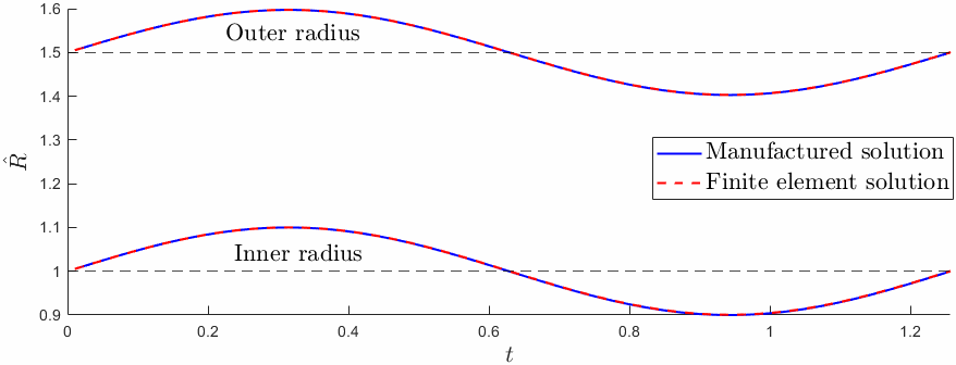
The deformed inner and outer radii of the shell against time.

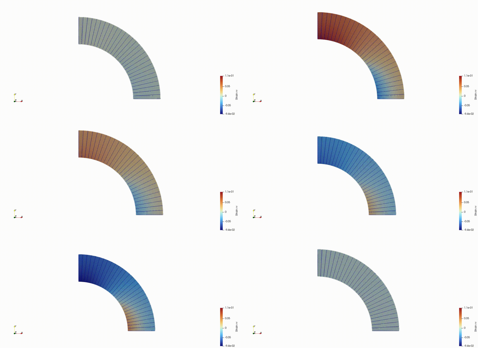
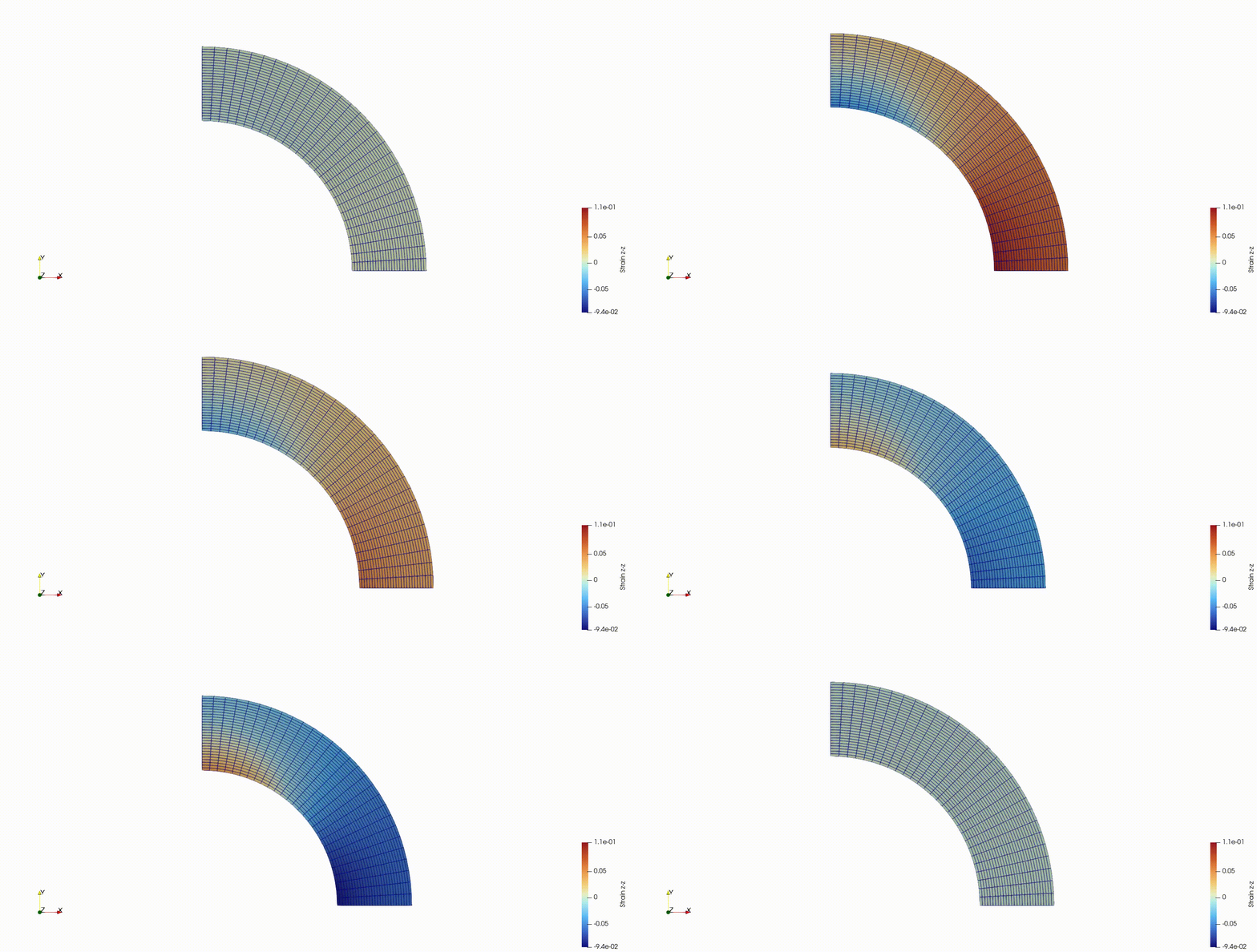
Also shown below are heatmaps of the components $\gamma_{rr}$ and $\gamma_{zz}$ of the Green-Lagrange strain tensor:

The rr-component (cylindrical coordinates) of the Green-Lagrange strain.

The zz-component of the Green-Lagrange strain.

Global parameters and functions

The namespace GlobalPhysicalVariables contains the material's Poisson ratio and the parameters , and $\omega$ that parameterise the manufactured displacement solution. The functions deformed_position_fct, deformed_velocity_fct and deformed_accel_fct are used to set the initial condition. The namespace also contains functions body_force_fct and traction_force_fct which define the forcing given by equations (1) and (2), respectively.

//=======start_namespace==========================================
/// Global physical variables
//================================================================
namespace GlobalPhysicalVariables
{
  // Poisson ratio
  double nu = 0.4;
 
  // Coefficient amplitudes for the manufactured solution
  double A0 = 0.05;
  double B0 = 0.05;
 
  // Oscillation frequency
  double omega = 5.0;
 
  // Get the principal stretches from the manufactured solution
  Vector<double> get_principal_stretches(const double& time, const double& r)
  {
    Vector<double> lambda(2);
    double A = A0 * sin(omega * time);
    double B = B0 * sin(omega * time);
    lambda[0] = 1.0 + A - 2.0 * B * pow(r, -3.0);
    lambda[1] = 1.0 + A + B * pow(r, -3.0);
    return lambda;
  }
 
  // Get derivatives of prinicipal stretches w.r.t. r
  Vector<double> get_principal_stretch_derivatives(const double& time,
                                                   const double& r)
  {
    Vector<double> dlambda_dr(2);
    double B = B0 * sin(omega * time);
    dlambda_dr[0] = 6.0 * B / pow(r, 4.0);
    dlambda_dr[1] = -3.0 * B / pow(r, 4.0);
    return dlambda_dr;
  }
 
  // Evaluate the deformed position
  void deformed_position_fct(const double& time,
                             const Vector<double>& xi,
                             Vector<double>& x)
  {
    double r = pow(xi[0] * xi[0] + xi[1] * xi[1], 0.5);
    double theta = atan2(xi[1], xi[0]);
    x[0] =
      xi[0] + (A0 * r + B0 * pow(r, -2.0)) * sin(omega * time) * cos(theta);
    x[1] =
      xi[1] + (A0 * r + B0 * pow(r, -2.0)) * sin(omega * time) * sin(theta);
  }
 
  // Evaluate the deformed position
  void deformed_velocity_fct(const double& time,
                             const Vector<double>& xi,
                             Vector<double>& x_dot)
  {
    double r = pow(xi[0] * xi[0] + xi[1] * xi[1], 0.5);
    double theta = atan2(xi[1], xi[0]);
    x_dot[0] =
      omega * (A0 * r + B0 * pow(r, -2.0)) * cos(omega * time) * cos(theta);
    x_dot[1] =
      omega * (A0 * r + B0 * pow(r, -2.0)) * cos(omega * time) * sin(theta);
  }
 
  // Evaluate the deformed position
  void deformed_accel_fct(const double& time,
                          const Vector<double>& xi,
                          Vector<double>& x_ddot)
  {
    double r = pow(xi[0] * xi[0] + xi[1] * xi[1], 0.5);
    double theta = atan2(xi[1], xi[0]);
    x_ddot[0] = -1.0 * omega * omega * (A0 * r + B0 * pow(r, -2.0)) *
                sin(omega * time) * cos(theta);
    x_ddot[1] = -1.0 * omega * omega * (A0 * r + B0 * pow(r, -2.0)) *
                sin(omega * time) * sin(theta);
  }
 
  // Body force function
  void body_force_fct(const double& time,
                      const Vector<double>& xi,
                      Vector<double>& b)
  {
    // Calculate the radial coordinate
    double r = pow(xi[0] * xi[0] + xi[1] * xi[1], 0.5);
    // Radial acceleration
    double accel =
      -1.0 * omega * omega * (A0 * r + B0 * pow(r, -2.0)) * sin(omega * time);
    // Principal stretches
    Vector<double> lambda = get_principal_stretches(time, r);
    // Jacobian
    double J = lambda[0] * lambda[1] * lambda[1];
    // Derivative of radial principal stretch and Jacobian w.r.t. r
    Vector<double> dlambda_dr = get_principal_stretch_derivatives(time, r);
    double dJdr = dlambda_dr[0] * lambda[1] * lambda[1] +
                  2.0 * lambda[0] * lambda[1] * dlambda_dr[1];
 
    // Dimensionless Lame parameters
    double mu_L = 1.0 / (2.0 * (1.0 + nu));
    double lambda_L = nu / ((1.0 + nu) * (1.0 - 2.0 * nu));
 
    // Evaluate the body force
    double b_spher =
      accel - mu_L * (dlambda_dr[0] + (2.0 / r) * (lambda[0] - lambda[1])) -
      lambda_L * dJdr / (J * lambda[0]) -
      (dlambda_dr[0] / (lambda[0] * lambda[0]) +
       (2.0 / r) * (1.0 / lambda[1] - 1.0 / lambda[0])) *
        (mu_L - lambda_L * log(J));
 
    double theta = atan2(xi[1], xi[0]);
    b[0] = b_spher * cos(theta);
    b[1] = b_spher * sin(theta);
  }
 
  // External traction force function
  void traction_force_fct(const double& time,
                          const Vector<double>& xi,
                          const Vector<double>& x,
                          const Vector<double>& n,
                          Vector<double>& traction)
  {
    // Calculate the (undeformed) radial coordinate
    double r = pow(xi[0] * xi[0] + xi[1] * xi[1], 0.5);
    // Principal stretches
    Vector<double> lambda = get_principal_stretches(time, r);
    // Jacobian
    double J = lambda[0] * lambda[1] * lambda[1];
 
    // Dimensionless Lame parameters
    double mu_L = 1.0 / (2.0 * (1.0 + nu));
    double lambda_L = nu / ((1.0 + nu) * (1.0 - 2.0 * nu));
 
    // Pressure required for the manufactured solution to work
    double ext_pressure =
      -1.0 * (mu_L * (lambda[0] * lambda[0] - 1.0) + lambda_L * log(J)) / J;
 
    // Return the traction
    traction[0] = -1.0 * ext_pressure * n[0];
    traction[1] = -1.0 * ext_pressure * n[1];
  }
} // namespace GlobalPhysicalVariables

A seperate namespace GlobalSimSettings then defines the simulation parameters such as the mesh dimensions, the number of timesteps in the run and the flag indicating if the solid pressure formulation is to be used.

//=======start_namespace==========================================
/// Global simulation settings
//================================================================
namespace GlobalSimSettings
{
  // Folder for output
  string result_folder = "RESLT";
 
  /// Flag for using a pressure formulation
  bool use_pressure_formulation = false;
 
  // Number of elements in radial direction
  unsigned n_radial = 14;
 
  // Number of elements in azimuthal direction
  unsigned n_azimuthal = 14;
 
  // Inner radius
  double a = 1.0;
 
  // Thickness
  double h = 0.5;
 
  // Number of timesteps
  unsigned Nsteps = 120;
 
  // Size of the timestep
  double dt;
} // namespace GlobalSimSettings

The mesh

As done in the previous tutorial, the mesh is constructed by upgrading the existing TwoDAnnularMesh to a solid mesh.

//======================start_mesh================================
/// Upgrade the mesh to a solidmesh.
/// Quarter-annulus in quadrant r>0, z>0
/// ntheta - no. elements in theta direction
/// nr - no. elements in the radial direction
/// a - Inner radius of annulus
/// h - thickness of annulus
//================================================================
template<class ELEMENT>
class ElasticTwoDAnnularMesh : public virtual TwoDAnnularMesh<ELEMENT>,
                               public virtual SolidMesh
{
public:
  /// Constructor: Build mesh and copy Eulerian coords to Lagrangian
  /// ones so that the initial configuration is the stress-free one.
  ElasticTwoDAnnularMesh<ELEMENT>(
    const unsigned& ntheta,
    const unsigned& nr,
    const double& a,
    const double& h,
    TimeStepper* time_stepper_pt = &Mesh::Default_TimeStepper)
    : RectangularQuadMesh<ELEMENT>(
        ntheta, nr, 1.0, 1.0, false, time_stepper_pt),
      TwoDAnnularMesh<ELEMENT>(false,
                               0.25,
                               ntheta,
                               nr,
                               a,
                               h,
                               MathematicalConstants::Pi,
                               time_stepper_pt)
  {
    // Make the current configuration the undeformed one by
    // setting the nodal Lagrangian coordinates to their current
    // Eulerian ones
    set_lagrangian_nodal_coordinates();
  }
};

The problem class

The problem class is relatively standard and is identical to the previous tutorial, execpt for the addition of the member functions set_initial_condition(), which sets the initial condition manually using functions provided in GlobalPhysicalVariables, and unsteady_run() which performs the time integration.

//==============start_problem=========================================
/// Axisymmetric compression of a finite thickness shell in cylindrical
/// polar coordiantes
//====================================================================
template<class ELEMENT>
class ShellProblem : public Problem
{
public:
  /// Constructor:
  ShellProblem();
 
  /// Destructor
  ~ShellProblem() {}
 
  /// Doc the solution
  void doc_solution();
 
  /// Set the initial condition
  void set_initial_condition();
 
  /// Run through the timesteps
  void unsteady_run();
 
private:
  /// Complete the problem setup (attach function/physical parameter pointers)
  void complete_problem_setup();
 
  /// Create the boundary elements
  void create_boundary_elements();
 
  /// Delete boundary elements and wipe the associated mesh
  void delete_boundary_elements()
  {
    // How many surface elements are in the surface mesh
    unsigned n_element = Surface_mesh_pt->nelement();
 
    // Loop over the surface elements
    for (unsigned e = 0; e < n_element; e++)
    {
      // Kill surface element
      delete Surface_mesh_pt->element_pt(e);
    }
 
    // Wipe the mesh
    Surface_mesh_pt->flush_element_and_node_storage();
  } // end of delete_boundary_elements
 
  /// Bulk mesh
  ElasticTwoDAnnularMesh<ELEMENT>* Bulk_mesh_pt;
 
  /// Surface mesh for traction force
  Mesh* Surface_mesh_pt;
 
  /// Pointer to constitutive law
  ConstitutiveLaw* Constitutive_law_pt;
 
  // DocInfo object
  DocInfo Doc_info;
};

The problem constructor

The constructor begins with assigning the output directory and setting Newmark<1> as the problem's timestepper. Following this, the bulk and surface meshes are created and the member function create_boundary_elements() is called to create traction elements on the outer boundary of the shell. complete_problem_setup() (discussed below) is called to complete the setup of the bulk and surface elements and assign Dirichlet boundary conditions. set_initial_condition() (also discussed below) is called to manually set an initial condition which is consistent with the manufactured solution.

//===============start_constructor========================================
/// Constructor for unstructured solid problem
//========================================================================
template<class ELEMENT>
ShellProblem<ELEMENT>::ShellProblem()
{
  // Set output directory
  Doc_info.set_directory(GlobalSimSettings::result_folder);
 
  // Initialise counter for solutions
  Doc_info.number() = 0;
 
  // Allocate the timestepper
  add_time_stepper_pt(new Newmark<1>);
 
  // Calculate the timestep size
  GlobalSimSettings::dt =
    2.0 * MathematicalConstants::Pi /
    (GlobalPhysicalVariables::omega * GlobalSimSettings::Nsteps);
 
  // Create the mesh: Quarter-annulus in the quadrant r>0, z>0.
  Bulk_mesh_pt =
    new ElasticTwoDAnnularMesh<ELEMENT>(GlobalSimSettings::n_azimuthal,
                                        GlobalSimSettings::n_radial,
                                        GlobalSimSettings::a,
                                        GlobalSimSettings::h,
                                        time_stepper_pt());
 
  // Create the surface mesh
  Surface_mesh_pt = new Mesh;
 
  // Create the boundary elements
  create_boundary_elements();
 
  // Add the two submeshes
  add_sub_mesh(Bulk_mesh_pt);
  add_sub_mesh(Surface_mesh_pt);
 
  // Combine all sub-meshes into a single mesh
  build_global_mesh();
 
  // Define a constitutive law from a strain energy density function.
  // Compressible Neo-Hookean
  StrainEnergyFunction* strain_energy_function_pt =
    new NeoHookean(&GlobalPhysicalVariables::nu);
  Constitutive_law_pt =
    new IsotropicStrainEnergyFunctionConstitutiveLaw(strain_energy_function_pt);
 
  // Complete the problem set up
  complete_problem_setup();
 
  // Set the initial condition consistently
  set_initial_condition();
 
  // Assign eqn numbers
  oomph_info << "Number of equations: " << assign_eqn_numbers() << std::endl;
} // end constructor

Completing the problem setup

To complete the problem setup, the pointers for the constutive law and body force function are passed to each of the bulk elements. The pointer to the traction force is then passed to each of the interface elements. Finally, the Dirichlet boundary conditions for the problem are set.

//========start_of_complete_problem_setup==================================
/// Assign function/parameter pointers, set boundary conditions etc.
//=========================================================================
template<class ELEMENT>
void ShellProblem<ELEMENT>::complete_problem_setup()
{
  // Determine number of bulk elements in mesh
  const unsigned n_element_bulk = Bulk_mesh_pt->nelement();
 
  // Loop over the bulk elements
  for (unsigned e = 0; e < n_element_bulk; e++)
  {
    // Upcast from GeneralisedElement to the present element
    ELEMENT* el_pt = dynamic_cast<ELEMENT*>(Bulk_mesh_pt->element_pt(e));
 
    // Set the constitutive law
    el_pt->constitutive_law_pt() = Constitutive_law_pt;
 
    // Set the traction function for applying pressure
    el_pt->body_force_fct_pt() = &GlobalPhysicalVariables::body_force_fct;
  } // End of loop over bulk elements
 
  // Determine number of 1D interface elements in mesh
  const unsigned n_interface_element = Surface_mesh_pt->nelement();
 
  // Loop over the interface elements
  for (unsigned e = 0; e < n_interface_element; e++)
  {
    // Upcast from GeneralisedElement to the present element
    AxisymmetricCylindricalSolidTractionElement<ELEMENT>* el_pt =
      dynamic_cast<AxisymmetricCylindricalSolidTractionElement<ELEMENT>*>(
        Surface_mesh_pt->element_pt(e));
 
    // Set the traction function for applying pressure
    el_pt->traction_fct_pt() = &GlobalPhysicalVariables::traction_force_fct;
 
  } // End of loop over interface elements
 
  // Set Dirichlet boundary conditions
  unsigned n_boundary_node = Bulk_mesh_pt->nboundary_node(1);
  for (unsigned n = 0; n < n_boundary_node; n++)
  {
    // Pin radial position on symmetry axis only
    Bulk_mesh_pt->boundary_node_pt(1, n)->pin_position(1);
  }
 
  n_boundary_node = Bulk_mesh_pt->nboundary_node(3);
  // Loop over nodes on fixed boundary
  for (unsigned n = 0; n < n_boundary_node; n++)
  {
    // Pin radial position on symmetry axis only
    Bulk_mesh_pt->boundary_node_pt(3, n)->pin_position(0);
  }
} // end complete_problem_setup

Setting the initial condition

Since this tutorial uses a manufactured solution, the nodal positions, velocities and accelerations are known at all times and so the initial condition can be set manually. The Newmark<1> timestepper stores the following values:

0: Displacement at time .
1: Displacement at time .
2: Velocity at time .
3: Acceleration at time .

These values are easily accessible using the functions deformed_position_fct, deformed_velocity_fct and deformed_accel_fct in the namespace GlobalPhysicalVariables.

//============start_of_set_initial_condition==============================
/// Given the form of the manufactured solution, this really only needs
/// doing for the velocity
//========================================================================
template<class ELEMENT>
void ShellProblem<ELEMENT>::set_initial_condition()
{
  // First initialize dt and set the weights
  initialise_dt(GlobalSimSettings::dt);
 
  // Loop over nodes
  unsigned n_node = Bulk_mesh_pt->nnode();
  for (unsigned n = 0; n < n_node; n++)
  {
    // Container for position/velocity/acceleration
    Vector<double> value(2);
 
    // Cast to (solid)node
    SolidNode* nod_pt = dynamic_cast<SolidNode*>(Bulk_mesh_pt->node_pt(n));
 
    // Get the undeformed position
    Vector<double> xi(2), x(2);
    xi[0] = nod_pt->lagrangian_position(0);
    xi[1] = nod_pt->lagrangian_position(1);
 
    // Set values of deformed position at the present and previous times
    GlobalPhysicalVariables::deformed_position_fct(0.0, xi, value);
    nod_pt->x(0, 0) = value[0];
    nod_pt->x(0, 1) = value[1];
    GlobalPhysicalVariables::deformed_position_fct(
      -1.0 * GlobalSimSettings::dt, xi, value);
    nod_pt->x(1, 0) = value[0];
    nod_pt->x(1, 1) = value[1];
 
    // Set the velocity at the previous time
    GlobalPhysicalVariables::deformed_velocity_fct(
      -1.0 * GlobalSimSettings::dt, xi, value);
    nod_pt->x(2, 0) = value[0];
    nod_pt->x(2, 1) = value[1];
 
    // Set the acceleration at the previous time
    GlobalPhysicalVariables::deformed_accel_fct(
      -1.0 * GlobalSimSettings::dt, xi, value);
    nod_pt->x(3, 0) = value[0];
    nod_pt->x(3, 1) = value[1];
  }
} // end set_initial_condition

The driver code

The driver code is relatively simple. Command line arguments for the material's Poisson ratio and the use_solid_pressure flag are specified. Following this, the problem is built and solved by calling the member function unsteady_run, which simply perfoms the Newton solve and output within a timestepping loop.

//===========start_main===================================================
/// Demonstrate how to solve an unstructured solid problem
//========================================================================
int main(int argc, char* argv[])
{
  // Store command line arguments
  CommandLineArgs::setup(argc, argv);
 
  string str_temp;
  CommandLineArgs::specify_command_line_flag(
    "--use_solid_pressure", &str_temp, "Use solid pressure");
 
  CommandLineArgs::specify_command_line_flag(
    "--poisson", &GlobalPhysicalVariables::nu, "Poisson");
 
  CommandLineArgs::specify_command_line_flag(
    "--Nsteps", &GlobalSimSettings::Nsteps, "Number of Steps");
 
  CommandLineArgs::parse_and_assign();
  CommandLineArgs::doc_specified_flags();
 
  istringstream(str_temp) >> std::boolalpha >>
    GlobalSimSettings::use_pressure_formulation;
 
  // Create the problem
  if (GlobalSimSettings::use_pressure_formulation)
  {
    // Build the problem with an additional degree of freedom for pressure
    ShellProblem<QAxisymmetricCylindricalPVDWithPressureElement> problem;
 
    // Perform time integration and docs
    problem.unsteady_run();
  }
  else
  {
    // Standard build
    ShellProblem<QAxisymmetricCylindricalPVDElement<3>> problem;
 
    // Perform time integration and docs
    problem.unsteady_run();
  }
} // end main

Source files for this tutorial

The source files for this tutorial are located in the directory: demo_drivers/axisym_solid/shell_unsteady/
The driver code is: demo_drivers/axisym_solid/shell_unsteady/shell_unsteady.cc

PDF file

A pdf version of this document is available. \